Data manipulation is crucial for transforming raw data into a more analyzable format, essential for uncovering patterns and ensuring accurate analysis. This chapter introduces the core techniques for data manipulation in Python, utilizing the Pandas library, a cornerstone for data handling within Python’s data science toolkit.
Python’s ecosystem is rich with libraries that facilitate not just data manipulation but comprehensive data analysis. Pandas, in particular, provides extensive functionality for data manipulation tasks including reading, cleaning, transforming, and summarizing data. Using real-world datasets, we will explore how to leverage Python for practical data manipulation tasks.
By the end of this chapter, you will learn to:
Import/export data from/to diverse sources.
Clean and preprocess data efficiently.
Transform and aggregate data to derive insights.
Merge and concatenate datasets from various origins.
Analyze real-world datasets using these techniques.
5.2 Example: NYC Crash Data
Consider a subset of the NYC Crash Data, which contains all NYC motor vehicle collisions data with documentation from NYC Open Data. We downloaded the crash data for the week of August 31, 2025, on September 11, 2025, in CSC format.
import numpy as npimport pandas as pd# Load the datasetfile_path ='data/nyc_crashes_lbdwk_2025.csv'df = pd.read_csv(file_path, dtype={'LATITUDE': np.float32,'LONGITUDE': np.float32,'ZIP CODE': str})# Replace column names: convert to lowercase and replace spaces with underscoresdf.columns = df.columns.str.lower().str.replace(' ', '_')# Check for missing valuesdf.isnull().sum()
# Replace invalid coordinates (latitude=0, longitude=0 or NaN) with NaNdf.loc[(df['latitude'] ==0) & (df['longitude'] ==0), ['latitude', 'longitude']] = pd.NAdf['latitude'] = df['latitude'].replace(0, pd.NA)df['longitude'] = df['longitude'].replace(0, pd.NA)# Drop the redundant `latitute` and `longitude` columnsdf = df.drop(columns=['location'])# Converting 'crash_date' and 'crash_time' columns into a single datetime columndf['crash_datetime'] = pd.to_datetime(df['crash_date'] +' '+ df['crash_time'], format='%m/%d/%Y %H:%M', errors='coerce')# Drop the original 'crash_date' and 'crash_time' columnsdf = df.drop(columns=['crash_date', 'crash_time'])
Let’s get some basic frequency tables of borough and zip_code, whose values could be used to check their validity against the legitmate values.
# Frequency table for 'borough' without filling missing valuesborough_freq = df['borough'].value_counts(dropna=False).reset_index()borough_freq.columns = ['borough', 'count']# Frequency table for 'zip_code' without filling missing valueszip_code_freq = df['zip_code'].value_counts(dropna=False).reset_index()zip_code_freq.columns = ['zip_code', 'count']zip_code_freq
zip_code
count
0
NaN
284
1
11207
33
2
11203
29
3
11212
23
4
11233
21
...
...
...
159
11379
1
160
10007
1
161
10308
1
162
11362
1
163
11694
1
164 rows × 2 columns
A comprehensive list of ZIP codes by borough can be obtained, for example, from the New York City Department of Health’s UHF Codes. We can use this list to check the validity of the zip codes in the data.
As it turns out, the collection of valid NYC zip codes differ from different sources. From United States Zip Codes, 10065 appears to be a valid NYC zip code. Under this circumstance, it might be safer to not remove any zip code from the data.
To be safe, let’s concatenate valid and invalid zips.
# Convert invalid ZIP codes to a set of stringsinvalid_zips_set =set(invalid_zip_freq['zip_code'].dropna().astype(str))# Convert all_valid_zips to a set of strings (if not already)valid_zips_set =set(map(str, all_valid_zips))# Merge both setsmerged_zips = invalid_zips_set | valid_zips_set # Union of both sets
Are missing in zip code and borough always co-occur?
# Check if missing values in 'zip_code' and 'borough' always co-occur# Count rows where both are missingmissing_cooccur = df[['zip_code', 'borough']].isnull().all(axis=1).sum()# Count total missing in 'zip_code' and 'borough', respectivelytotal_missing_zip_code = df['zip_code'].isnull().sum()total_missing_borough = df['borough'].isnull().sum()# If missing in both columns always co-occur, the number of missing# co-occurrences should be equal to the total missing in either columnnp.array([missing_cooccur, total_missing_zip_code, total_missing_borough])
array([284, 284, 284])
Are there cases where zip_code and borough are missing but the geo codes are not missing? If so, fill in zip_code and borough using the geo codes by reverse geocoding.
First make sure geopy is installed.
pip install geopy
Now we use module Nominatim in package geopy to reverse geocode.
from geopy.geocoders import Nominatimimport time# Initialize the geocoder; the `user_agent` is your identifier # when using the service. Be mindful not to crash the server# by unlimited number of queries, especially invalid code.geolocator = Nominatim(user_agent="jyGeopyTry")
We write a function to do the reverse geocoding given lattitude and longitude.
# Function to fill missing zip_codedef get_zip_code(latitude, longitude):try: location = geolocator.reverse((latitude, longitude), timeout=10)if location: address = location.raw['address'] zip_code = address.get('postcode', None)return zip_codeelse:returnNoneexceptExceptionas e:print(f"Error: {e} for coordinates {latitude}, {longitude}")returnNonefinally: time.sleep(1) # Delay to avoid overwhelming the service
Let’s try it out:
# Example usagelatitude =40.730610longitude =-73.935242get_zip_code(latitude, longitude)
'11101'
The function get_zip_code can then be applied to rows where zip code is missing but geocodes are not to fill the missing zip code.
Once zip code is known, figuring out burough is simple because valid zip codes from each borough are known.
5.3 Accessing Census Data
The U.S. Census Bureau provides extensive demographic, economic, and social data through multiple surveys, including the decennial Census, the American Community Survey (ACS), and the Economic Census. These datasets offer valuable insights into population trends, economic conditions, and community characteristics at multiple geographic levels.
There are multiple ways to access Census data. For example:
Census API: The Census API allows programmatic access to various datasets. It supports queries for different geographic levels and time periods.
data.census.gov: The official web interface for searching and downloading Census data.
IPUMS USA: Provides harmonized microdata for longitudinal research. Available at IPUMS USA.
NHGIS: Offers historical Census data with geographic information. Visit NHGIS.
In addition, Python tools simplify API access and data retrieval.
5.3.1 Python Tools for Accessing Census Data
Several Python libraries facilitate Census data retrieval:
census: A high-level interface to the Census API, supporting ACS and decennial Census queries. See census on PyPI.
censusdis: Provides richer functionality: automatic discovery of variables, geographies, and datasets. Helpful if you don’t want to manually look up variable codes. See censusdis on PyPI.
us: Often used alongside census libraries to handle U.S. state and territory information (e.g., FIPS codes). See us on PyPI.
5.3.2 Zip-Code Level for NYC Crash Data
Now that we have NYC crash data, we might want to analyze patterns at the zip-code level to understand whether certain demographic or economic factors correlate with traffic incidents. While the crash dataset provides details about individual accidents, such as location, time, and severity, it does not contain contextual information about the neighborhoods where these crashes occur.
To perform meaningful zip-code-level analysis, we need additional data sources that provide relevant demographic, economic, and geographic variables. For example, understanding whether high-income areas experience fewer accidents, or whether population density influences crash frequency, requires integrating Census data. Key variables such as population size, median household income, employment rate, and population density can provide valuable context for interpreting crash trends across different zip codes.
Since the Census Bureau provides detailed estimates for these variables at the zip-code level, we can use the Census API or other tools to retrieve relevant data and merge it with the NYC crash dataset. To access the Census API, you need an API key, which is free and easy to obtain. Visit the Census API Request page and submit your email address to receive a key. Once you have the key, you must include it in your API requests to access Census data. The following demonstration assumes that you have registered, obtained your API key, and saved it in a file called censusAPIkey.txt.
# Import modulesimport matplotlib.pyplot as pltimport pandas as pdimport geopandas as gpdfrom census import Censusfrom us import statesimport osimport ioapi_key =open("censusAPIkey.txt").read().strip()c = Census(api_key)
Suppose that we want to get some basic info from ACS data of the year of 2024 for all the NYC zip codes. The variable names can be found in the ACS variable documentation.
ACS_YEAR =2024ACS_DATASET ="acs/acs5"# Important ACS variables (including land area for density calculation)ACS_VARIABLES = {"B01003_001E": "Total Population","B19013_001E": "Median Household Income","B02001_002E": "White Population","B02001_003E": "Black Population","B02001_005E": "Asian Population","B15003_022E": "Bachelor’s Degree Holders","B15003_025E": "Graduate Degree Holders","B23025_002E": "Labor Force","B23025_005E": "Unemployed","B25077_001E": "Median Home Value"}# Convert set to list of stringsmerged_zips =list(map(str, merged_zips))
Let’s set up the query to request the ACS data, and process the returned data.
We could save the ACS data df_acs in feather format (see next Section).
df_acs.to_feather("data/acs2023.feather")
The population density could be an important factor for crash likelihood. To obtain the population densities, we need the areas of the zip codes. The shape files can be obtained from NYC Open Data.
import requestsimport zipfileimport geopandas as gpd# Define the NYC MODZCTA shapefile URL and extraction directoryshapefile_url ="https://data.cityofnewyork.us/api/geospatial/pri4-ifjk?method=export&format=Shapefile"extract_dir ="MODZCTA_Shapefile"# Create the directory if it doesn't existos.makedirs(extract_dir, exist_ok=True)# Step 1: Download and extract the shapefileprint("Downloading MODZCTA shapefile...")response = requests.get(shapefile_url)with zipfile.ZipFile(io.BytesIO(response.content), "r") as z: z.extractall(extract_dir)print(f"Shapefile extracted to: {extract_dir}")
Downloading MODZCTA shapefile...
Shapefile extracted to: MODZCTA_Shapefile
Now we process the shape file to calculate the areas of the polygons.
# Step 2: Automatically detect the correct .shp fileshapefile_path =Noneforfilein os.listdir(extract_dir):iffile.endswith(".shp"): shapefile_path = os.path.join(extract_dir, file)break# Use the first .shp file foundifnot shapefile_path:raiseFileNotFoundError("No .shp file found in extracted directory.")print(f"Using shapefile: {shapefile_path}")# Step 3: Load the shapefile into GeoPandasgdf = gpd.read_file(shapefile_path)# Step 4: Convert to CRS with meters for accurate area calculationgdf = gdf.to_crs(epsg=3857)# Step 5: Compute land area in square milesgdf['land_area_sq_miles'] = gdf['geometry'].area /2_589_988.11# 1 square mile = 2,589,988.11 square metersprint(gdf[['modzcta', 'land_area_sq_miles']].head())
# Merge ACS data (`df_acs`) directly with MODZCTA land area (`gdf`)gdf = gdf.merge(df_acs, left_on='modzcta', right_on='ZIP Code', how='left')# Calculate Population Density (people per square mile)gdf['popdensity_per_sq_mile'] = ( gdf['Total Population'] / gdf['land_area_sq_miles'] )# Display first few rowsprint(gdf[['modzcta', 'Total Population', 'land_area_sq_miles','popdensity_per_sq_mile']].head())
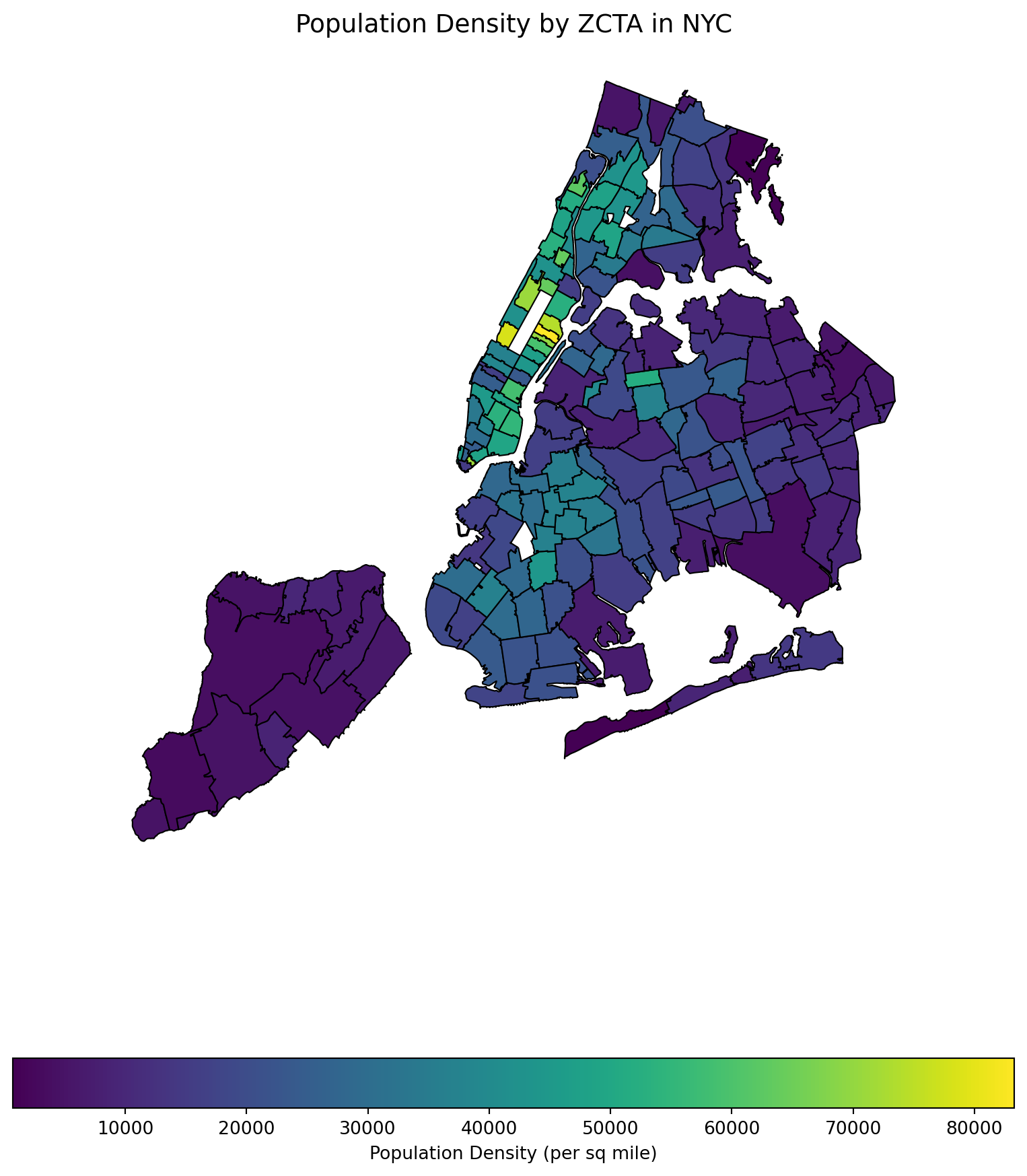
import matplotlib.pyplot as pltimport geopandas as gpd# Set up figure and axisfig, ax = plt.subplots(figsize=(10, 12))# Plot the choropleth mapgdf.plot(column='popdensity_per_sq_mile', cmap='viridis', # Use a visually appealing color map linewidth=0.8, edgecolor='black', legend=True, legend_kwds={'label': "Population Density (per sq mile)",'orientation': "horizontal"}, ax=ax)# Add a titleax.set_title("Population Density by ZCTA in NYC", fontsize=14)# Remove axesax.set_xticks([])ax.set_yticks([])ax.set_frame_on(False)# Show the plotplt.show()
5.4 Cross-platform Data Format Arrow
The CSV format (and related formats like TSV - tab-separated values) for data tables is ubiquitous, convenient, and can be read or written by many different data analysis environments, including spreadsheets. An advantage of the textual representation of the data in a CSV file is that the entire data table, or portions of it, can be previewed in a text editor. However, the textual representation can be ambiguous and inconsistent. The format of a particular column: Boolean, integer, floating-point, text, factor, etc. must be inferred from text representation, often at the expense of reading the entire file before these inferences can be made. Experienced data scientists are aware that a substantial part of an analysis or report generation is often the “data cleaning” involved in preparing the data for analysis. This can be an open-ended task — it required numerous trial-and-error iterations to create the list of different missing data representations we use for the sample CSV file and even now we are not sure we have them all.
To read and export data efficiently, leveraging the Apache Arrow library can significantly improve performance and storage efficiency, especially with large datasets. The IPC (Inter-Process Communication) file format in the context of Apache Arrow is a key component for efficiently sharing data between different processes, potentially written in different programming languages. Arrow’s IPC mechanism is designed around two main file formats:
Stream Format: For sending an arbitrary length sequence of Arrow record batches (tables). The stream format is useful for real-time data exchange where the size of the data is not known upfront and can grow indefinitely.
File (or Feather) Format: Optimized for storage and memory-mapped access, allowing for fast random access to different sections of the data. This format is ideal for scenarios where the entire dataset is available upfront and can be stored in a file system for repeated reads and writes.
Apache Arrow provides a columnar memory format for flat and hierarchical data, optimized for efficient data analytics. It can be used in Python through the pyarrow package. Here’s how you can use Arrow to read, manipulate, and export data, including a demonstration of storage savings.
First, ensure you have pyarrow installed on your computer (and preferrably, in your current virtual environment):
pip install pyarrow
Feather is a fast, lightweight, and easy-to-use binary file format for storing data frames, optimized for speed and efficiency, particularly for IPC and data sharing between Python and R or Julia.
The following code processes the cleaned data in CSV format from Mohammad Mundiwala and write out in Arrow format.
#| eval: falseimport pandas as pd# Read CSV, ensuring 'zip_code' is string and 'crash_datetime' is parsed as datetimedf = pd.read_csv('data/nyc_crashes_cleaned_mm.csv', dtype={'zip_code': str}, parse_dates=['crash_datetime'])# Drop the 'date' and 'time' columnsdf = df.drop(columns=['crash_date', 'crash_time'])# Move 'crash_datetime' to the first columndf = df[['crash_datetime'] + df.drop(columns=['crash_datetime']).columns.tolist()]df['zip_code'] = df['zip_code'].astype(str).str.rstrip('.0')df = df.sort_values(by='crash_datetime')df.to_feather('nyccrashes_cleaned.feather')
Let’s compare the file sizes of the feather format and the CSV format.
import os# File pathscsv_file ='data/nyccrashes_2024w0630_by20250212.csv'feather_file ='data/nyccrashes_cleaned.feather'# Get file sizes in bytescsv_size = os.path.getsize(csv_file)feather_size = os.path.getsize(feather_file)# Convert bytes to a more readable format (e.g., MB)csv_size_mb = csv_size / (1024*1024)feather_size_mb = feather_size / (1024*1024)# Print the file sizesprint(f"CSV file size: {csv_size_mb:.2f} MB")print(f"Feather file size: {feather_size_mb:.2f} MB")