5  Data Import/Export

Working with data is a fundamental aspect of data science in Python, with data import and export being crucial skills. Throughout, we will use the 311 service request data for illustrations, downloaded from the NYC Open Data as a csv file.

5.1 Using the Pandas Package

The pandas library simplifies data manipulation and analysis. It’s especially handy for dealing with CSV files.

import pandas as pd

# Define the file name
csvnm = "data/rodent_2022-2023.csv"

# Specify the strings that indicate missing values
# Q: How would you know these?
na_values = [
    "",
    "0 Unspecified",
    "N/A",
    "na",
    "na na",
    "Unspecified",
    "UNKNOWN",
]

def custom_date_parser(x):
    return pd.to_datetime(x, format="%m/%d/%Y %I:%M:%S %p", errors='coerce')

# Read the CSV file
df = pd.read_csv(
    csvnm,
    na_values = na_values,
    parse_dates = ['Created Date', 'Closed Date'], 
    date_parser = custom_date_parser,
    dtype = {'Latitude': 'float32', 'Longitude': 'float32'},
)

# Strip leading and trailing whitespace from the column names
df.columns = df.columns.str.strip()
df.columns = df.columns.str.replace(' ', '_', regex = False).str.lower()

# Drop the 'Location' since it is redundant
# df.drop(columns=['Location'], inplace=True)
/var/folders/cq/5ysgnwfn7c3g0h46xyzvpj800000gn/T/ipykernel_27231/754040398.py:22: FutureWarning:

The argument 'date_parser' is deprecated and will be removed in a future version. Please use 'date_format' instead, or read your data in as 'object' dtype and then call 'to_datetime'.

The pandas package also provides some utility functions for quick summaries about the data frame.

df.shape
df.describe()
df.isnull().sum()
unique_key                            0
created_date                          0
closed_date                        2787
agency                                0
agency_name                           0
complaint_type                        0
descriptor                            0
location_type                         0
incident_zip                          0
incident_address                      0
street_name                           0
cross_street_1                       90
cross_street_2                       55
intersection_street_1               104
intersection_street_2                69
address_type                          0
city                               1384
landmark                           3820
facility_type                     82869
status                                2
due_date                          82869
resolution_description             2787
resolution_action_updated_date     2787
community_board                       8
bbl                                2914
borough                               8
x_coordinate_(state_plane)          520
y_coordinate_(state_plane)          520
open_data_channel_type                0
park_facility_name                82869
park_borough                          8
vehicle_type                      82869
taxi_company_borough              82869
taxi_pick_up_location             82869
bridge_highway_name               82869
bridge_highway_direction          82869
road_ramp                         82869
bridge_highway_segment            82869
latitude                            520
longitude                           520
location                            520
zip_codes                           622
community_districts                 526
borough_boundaries                  526
city_council_districts              526
police_precincts                    526
police_precinct                     526
dtype: int64

What are the unique values of descriptor?

df.descriptor.unique()
array(['Rat Sighting', 'Mouse Sighting', 'Condition Attracting Rodents',
       'Signs of Rodents', 'Rodent Bite - PCS Only'], dtype=object)

5.2 Filling Missing Values

If geocodes are available but zip code is missing, we can use reverse geocoding to fill the zip code. This process involves querying a geocoding service with latitude and longitude to get the corresponding address details, including the ZIP code. This can be done with package geopy, which needs to be installed first: pip install geopy.

import pandas as pd
from geopy.geocoders import Nominatim
from geopy.exc import GeocoderTimedOut, GeocoderServiceError

# Initialize the geocoder
geolocator = Nominatim(user_agent="geoapiExercises")

# Function for reverse geocoding
def reverse_geocode(lat, lon):
    try:
        location = geolocator.reverse((lat, lon), exactly_one=True)
        address = location.raw.get('address', {})
        zip_code = address.get('postcode')
        return zip_code
    except (GeocoderTimedOut, GeocoderServiceError):
        # Handle errors or timeouts
        return None

# Apply reverse geocoding to fill missing ZIP codes
for index, row in df.iterrows():
    if pd.isnull(row['incident_zip']) and pd.notnull(row['latitude']) and pd.notnull(row['longitude']):
        df.at[index, 'incident_zip'] = reverse_geocode(row['latitude'], row['longitude'])

# Note: This can be slow for large datasets due to API rate
# limits and network latency

5.3 Using Appache Arrow Library

To read and export data efficiently, leveraging the Apache Arrow library can significantly improve performance and storage efficiency, especially with large datasets. The IPC (Inter-Process Communication) file format in the context of Apache Arrow is a key component for efficiently sharing data between different processes, potentially written in different programming languages. Arrow’s IPC mechanism is designed around two main file formats:

  • Stream Format: For sending an arbitrary length sequence of Arrow record batches (tables). The stream format is useful for real-time data exchange where the size of the data is not known upfront and can grow indefinitely.
  • File (or Feather) Format: Optimized for storage and memory-mapped access, allowing for fast random access to different sections of the data. This format is ideal for scenarios where the entire dataset is available upfront and can be stored in a file system for repeated reads and writes.

Apache Arrow provides a columnar memory format for flat and hierarchical data, optimized for efficient data analytics. It can be used in Python through the pyarrow package. Here’s how you can use Arrow to read, manipulate, and export data, including a demonstration of storage savings.

First, ensure you have pyarrow installed on your computer (and preferrably, in your current virtual environment):

pip install pyarrow

Feather is a fast, lightweight, and easy-to-use binary file format for storing data frames, optimized for speed and efficiency, particularly for IPC and data sharing between Python and R.

df.to_feather('data/rodent_2022-2023.feather')

Read the feather file back in:

dff = pd.read_feather("data/rodent_2022-2023.feather")
dff.shape
(82869, 47)

Benefits of Using Feather:

  • Efficiency: Feather is designed to support fast reading and writing of data frames, making it ideal for analytical workflows that need to exchange large datasets between Python and R.
  • Compatibility: Maintains data type integrity across Python and R, ensuring that numbers, strings, and dates/times are correctly handled and preserved.
  • Simplicity: The API for reading and writing Feather files is straightforward, making it accessible to users with varying levels of programming expertise.

By using Feather format for data storage, you leverage a modern approach optimized for speed and compatibility, significantly enhancing the performance of data-intensive applications.

5.4 Accessing the Census Data with uszipcode

First, ensure the DataFrame (df) is ready for merging with census data. Specifically, check that the incident_zip column is clean and consistent.

print(df['incident_zip'].isnull().sum())
# Standardize to 5-digit codes, if necessary
df['incident_zip'] = df['incident_zip'].astype(str).str.zfill(5) 
0

We can use the uszipcode package to get basic demographic data for each zip code. For more detailed or specific census data, using the CensusData package or direct API calls to the Census Bureau’s API.

The uszipcode package provides a range of information about ZIP codes in the United States. When you query a ZIP code using uszipcode, you can access various attributes related to demographic data, housing, geographic location, and more. Here are some of the key variables available at the ZIP code level:

emographic Information

  • population: The total population.
  • population_density: The population per square kilometer.
  • housing_units: The total number of housing units.
  • occupied_housing_units: The number of occupied housing units.
  • median_home_value: The median value of homes.
  • median_household_income: The median household income.
  • age_distribution: A breakdown of the population by age.

Geographic Information

  • zipcode: The ZIP code.
  • zipcode_type: The type of ZIP code (e.g., Standard, PO Box).
  • major_city: The major city associated with the ZIP code.
  • post_office_city: The city name recognized by the U.S. Postal Service.
  • common_city_list: A list of common city names for the ZIP code.
  • county: The county in which the ZIP code is located.
  • state: The state in which the ZIP code is located.
  • lat: The latitude of the approximate center of the ZIP code.
  • lng: The longitude of the approximate center of the ZIP code.
  • timezone: The timezone of the ZIP code.

Economic and Housing Data

  • land_area_in_sqmi: The land area in square miles.
  • water_area_in_sqmi: The water area in square miles.
  • occupancy_rate: The rate of occupancy for housing units.
  • median_age: The median age of the population.

Install the uszipcode package into the current virtual environment by pip install uszipcode.

Now let’s work on the rodent sightings data.

We will first clean the incident_zip column to ensure it only contains valid ZIP codes. Then, we will use a vectorized approach to fetch the required data for each unique ZIP code and merge this information back into the original DataFrame.

# Remove rows where 'incident_zip' is missing or not a valid ZIP code format
valid_zip_df = df.dropna(subset=['incident_zip']).copy()
valid_zip_df['incident_zip'] = valid_zip_df['incident_zip'].astype(str).str.zfill(5)
unique_zips = valid_zip_df['incident_zip'].unique()

Since uszipcode doesn’t inherently support vectorized operations for multiple ZIP code queries, we’ll optimize the process by querying each unique ZIP code once, then merging the results with the original DataFrame. This approach minimizes redundant queries for ZIP codes that appear multiple times.

from uszipcode import SearchEngine

# Initialize the SearchEngine
search = SearchEngine()

# Fetch median home value and median household income for each unique ZIP code
zip_data = []
zip_data = []
for zip_code in unique_zips:
    result = search.by_zipcode(zip_code)
    if result:  # Check if the result is not None
        zip_data.append({
            "incident_zip": zip_code,
            "median_home_value": result.median_home_value,
            "median_household_income": result.median_household_income
        })
    else:  # Handle the case where the result is None
        zip_data.append({
            "incident_zip": zip_code,
            "median_home_value": None,
            "median_household_income": None
        })

# Convert to DataFrame
zip_info_df = pd.DataFrame(zip_data)

# Merge this info back into the original DataFrame based on 'incident_zip'
merged_df = pd.merge(valid_zip_df, zip_info_df, how="left", on="incident_zip")

merged_df.columns
/Users/junyan/work/teaching/ids-s24/ids-s24/.myvenv/lib/python3.12/site-packages/fuzzywuzzy/fuzz.py:11: UserWarning:

Using slow pure-python SequenceMatcher. Install python-Levenshtein to remove this warning
Index(['unique_key', 'created_date', 'closed_date', 'agency', 'agency_name',
       'complaint_type', 'descriptor', 'location_type', 'incident_zip',
       'incident_address', 'street_name', 'cross_street_1', 'cross_street_2',
       'intersection_street_1', 'intersection_street_2', 'address_type',
       'city', 'landmark', 'facility_type', 'status', 'due_date',
       'resolution_description', 'resolution_action_updated_date',
       'community_board', 'bbl', 'borough', 'x_coordinate_(state_plane)',
       'y_coordinate_(state_plane)', 'open_data_channel_type',
       'park_facility_name', 'park_borough', 'vehicle_type',
       'taxi_company_borough', 'taxi_pick_up_location', 'bridge_highway_name',
       'bridge_highway_direction', 'road_ramp', 'bridge_highway_segment',
       'latitude', 'longitude', 'location', 'zip_codes', 'community_districts',
       'borough_boundaries', 'city_council_districts', 'police_precincts',
       'police_precinct', 'median_home_value', 'median_household_income'],
      dtype='object')

5.5 Accessing ACS Data

This section was written by Abigail Mori.

5.5.1 Introduction

Hi! My name is Abigail Mori and I am a current senior, graduating this May. This past summer I worked with the UConn’s Center for Voting Technology Research. We used ACS data to analyze ease of voting within Connecticut. Though, I only used sql and never had to access this data through python. I am excited to show what I’ve learned over the past couple weeks.

5.5.2 Installation

In order to properly access ACS data we will need make sure we have installed cenpy and geodatasets. Cenpy is a package that “automatically discovers US Census Bureau API endpoints and exposes them to Python in a consistent fashion.” Geodatasets “contains an API on top of a JSON with metadata of externally hosted datasets containing geospatial information useful for illustrative and educational purposes.” Both of these modules are dependent on pandas.

5.5.3 Accessing ACS Data

There are many different kinds of census data, one of which is ACS (American Community Survery) data. The ACS data is made up of a “wide range of social, economic, demographic, and housing charateristics.” There are multiple ways to access this data using Python. I will examine one way using cenpy.

For much of work I referenced a cenpy API reference page (https://cenpy-devs.github.io/cenpy/api.html)

import warnings
warnings.simplefilter(action='ignore', category=FutureWarning)
import cenpy as cen
import geodatasets
# Set a variable to all tables in the The American Community Survey from
#  the Census Bureau
acs = cen.products.ACS()
# Filter through acs tables based on specific variables
print(acs.filter_tables('RACE', by='description'))
# Once you select your desired table you can add more specific parameters, 
# in this case I chose to do so by state
connecticut = cen.products.ACS(2019).from_state('Connecticut',
 variables= 'B02001')
print(connecticut.head())
nevada = cen.products.ACS(2019).from_state('Nevada', 
variables= 'B02001')
print(nevada.head())
                                                  description  \
table_name                                                      
B02001                                                   RACE   
B02008      WHITE ALONE OR IN COMBINATION WITH ONE OR MORE...   
B02009      BLACK OR AFRICAN AMERICAN ALONE OR IN COMBINAT...   
B02010      AMERICAN INDIAN AND ALASKA NATIVE ALONE OR IN ...   
B02011      ASIAN ALONE OR IN COMBINATION WITH ONE OR MORE...   
B02012      NATIVE HAWAIIAN AND OTHER PACIFIC ISLANDER ALO...   
B02013      SOME OTHER RACE ALONE OR IN COMBINATION WITH O...   
B03002                      HISPANIC OR LATINO ORIGIN BY RACE   
B25006                                    RACE OF HOUSEHOLDER   
B98013      TOTAL POPULATION COVERAGE RATE BY WEIGHTING RA...   
B99021                                     ALLOCATION OF RACE   
C02003                                          DETAILED RACE   

                                                      columns  
table_name                                                     
B02001      [B02001_001E, B02001_002E, B02001_003E, B02001...  
B02008                                          [B02008_001E]  
B02009                                          [B02009_001E]  
B02010                                          [B02010_001E]  
B02011                                          [B02011_001E]  
B02012                                          [B02012_001E]  
B02013                                          [B02013_001E]  
B03002      [B03002_001E, B03002_002E, B03002_003E, B03002...  
B25006      [B25006_001E, B25006_002E, B25006_003E, B25006...  
B98013      [B98013_001E, B98013_002E, B98013_003E, B98013...  
B99021                [B99021_001E, B99021_002E, B99021_003E]  
C02003      [C02003_001E, C02003_002E, C02003_003E, C02003...  
         GEOID                                           geometry  \
0  09001010400  POLYGON ((-8201121.400 5017141.610, -8201100.1...   
1  09001010600  POLYGON ((-8196750.330 5017084.050, -8196748.9...   
2  09001010300  POLYGON ((-8200317.120 5018093.350, -8200295.0...   
3  09001011300  POLYGON ((-8199823.530 5012413.050, -8199813.0...   
4  09001020500  POLYGON ((-8193009.330 5026964.430, -8192869.1...   

   B02001_001E  B02001_002E  B02001_003E  B02001_004E  B02001_005E  \
0       5799.0       4698.0        531.0         17.0        346.0   
1       2062.0       1518.0        282.0          0.0        145.0   
2       3780.0       3305.0        123.0          0.0        247.0   
3       3416.0       2530.0         65.0          8.0        154.0   
4       4886.0       4236.0        232.0        117.0        114.0   

   B02001_006E  B02001_007E  B02001_008E  B02001_009E  B02001_010E  \
0          0.0        143.0         64.0          0.0         64.0   
1         11.0         33.0         73.0          7.0         66.0   
2          0.0         10.0         95.0         16.0         79.0   
3         20.0        408.0        231.0         67.0        164.0   
4         15.0          0.0        172.0          0.0        172.0   

                                              NAME state county   tract  
0  Census Tract 104, Fairfield County, Connecticut    09    001  010400  
1  Census Tract 106, Fairfield County, Connecticut    09    001  010600  
2  Census Tract 103, Fairfield County, Connecticut    09    001  010300  
3  Census Tract 113, Fairfield County, Connecticut    09    001  011300  
4  Census Tract 205, Fairfield County, Connecticut    09    001  020500  
         GEOID                                           geometry  \
0  32031002613  POLYGON ((-13358452.220 4827161.350, -13358451...   
1  32031003308  POLYGON ((-13359059.470 4760834.720, -13357433...   
2  32031980200  POLYGON ((-13358521.900 4802740.580, -13358516...   
3  32031002407  POLYGON ((-13346382.740 4800296.200, -13346335...   
4  32031001105  POLYGON ((-13343276.140 4791951.280, -13343275...   

   B02001_001E  B02001_002E  B02001_003E  B02001_004E  B02001_005E  \
0       5830.0       5387.0        140.0         35.0         74.0   
1       2155.0       1976.0          0.0         35.0         74.0   
2          0.0          0.0          0.0          0.0          0.0   
3       4151.0       3025.0         87.0        114.0        671.0   
4       3819.0       3434.0         67.0          0.0        233.0   

   B02001_006E  B02001_007E  B02001_008E  B02001_009E  B02001_010E  \
0         25.0         61.0        108.0          0.0        108.0   
1          9.0          4.0         57.0         12.0         45.0   
2          0.0          0.0          0.0          0.0          0.0   
3         29.0         77.0        148.0         55.0         93.0   
4         14.0         16.0         55.0          0.0         55.0   

                                        NAME state county   tract  
0  Census Tract 26.13, Washoe County, Nevada    32    031  002613  
1  Census Tract 33.08, Washoe County, Nevada    32    031  003308  
2   Census Tract 9802, Washoe County, Nevada    32    031  980200  
3  Census Tract 24.07, Washoe County, Nevada    32    031  002407  
4  Census Tract 11.05, Washoe County, Nevada    32    031  001105  

Each columns meanings can be found here: https://api.census.gov/data/2019/acs/acs1/variables.html and https://www.census.gov/programs-surveys/acs/technical-documentation /table-shells.2019.html#list-tab-79594641

B02001_001E: Total
B02001_002E White alone
B02001_003E Black or African American alone
B02001_004E American Indian and Alaska Native alone
B02001_005E Asian alone
B02001_006E Native Hawaiian and Other Pacific Islander alone
B02001_007E Some other race alone
B02001_008E Two or more races
B02001_009E Two races including Some other race
B02001_010E Two races excluding Some other race, and three or more races

5.5.4 Visualizing

Cenpy returns users with datasets based on specifications, like RACE. Some of the columns include: geiod, geometry, name, state, county, and tract. The geometry is made up of Polygons which then can be used to make a map with matplotlib Since, cenpy provides a table of type: geopandas.geodataframe.GeoDataFrame. GeoPandas provides a high-level interface to the matplotlib library for making maps.

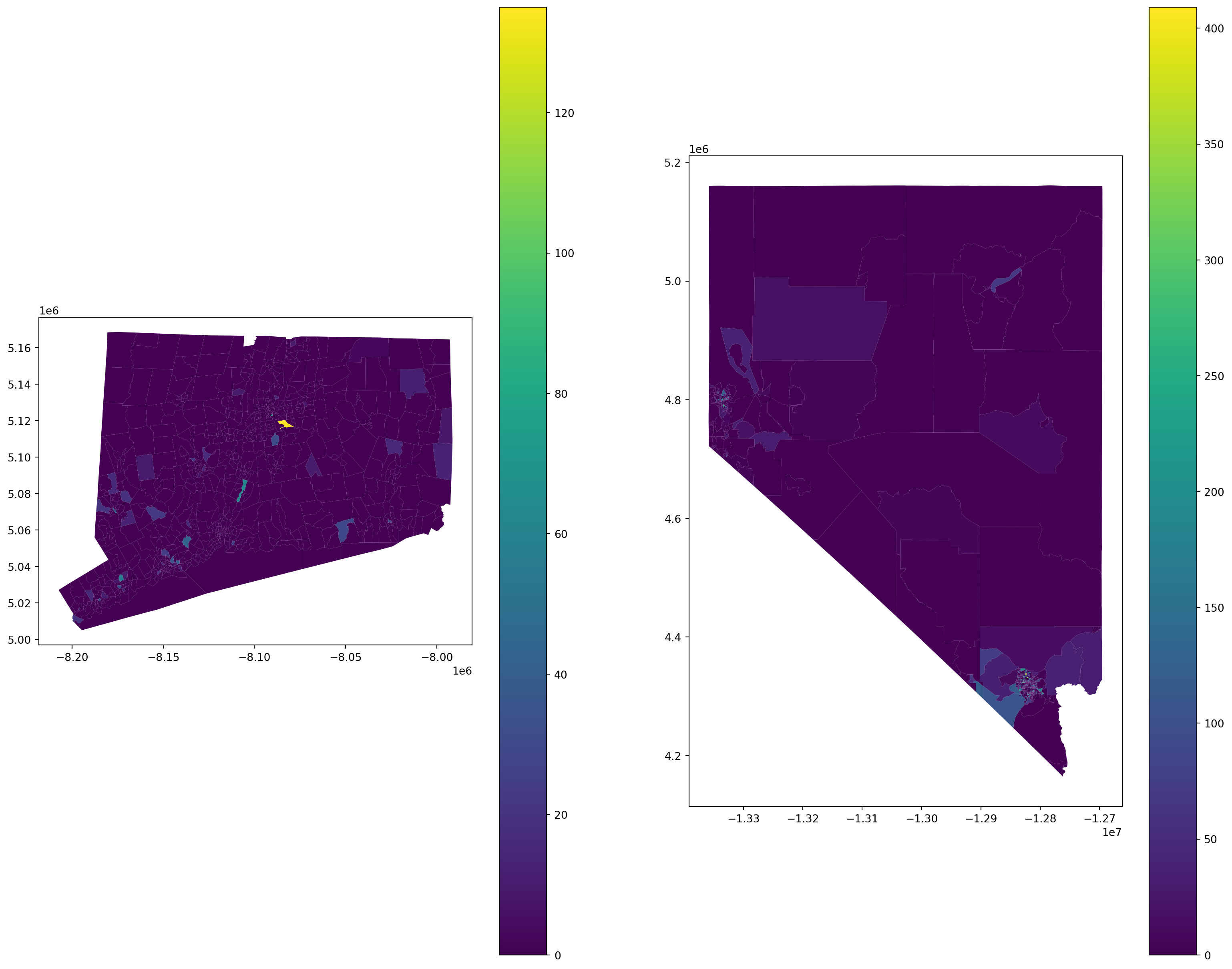
Below, I show maps of Connecticut and Nevada which display the populations of Native Hawaiians and other Pacific Islanders by census tract.

import matplotlib.pyplot as plt
import geopandas
import pandas as pd
fig, (ax1,ax2) = plt.subplots(nrows=1, ncols=2, 
figsize=(20, 16))

#B02001_006E: total number of Native Hawaiians and other Pacific Islanders
ax1 = connecticut.plot('B02001_006E', ax = ax1, cmap = 'viridis', legend = True)
ax2 = nevada.plot('B02001_006E', ax = ax2, cmap = 'viridis', legend = True)

5.5.5 Further Analysis

ACS data can allow individuals to see discrepancies in voting accessability. For instance, we can look at correlation between a poverty level and education in a specific state.

We can access this data doing the same search method as above.

Like before we filter through the tables to access our desired data. In this instance I chose to select data concerning poverty and education in Connecticut.

print(acs.filter_tables('POVERTY', by='description'))
# B17001: Poverty status in the past 12 months 
poverty_ct = cen.products.ACS(2019).from_state('Connecticut', 
variables = 'B17001')
poverty_ct.head()
                                                  description  \
table_name                                                      
B05010      RATIO OF INCOME TO POVERTY LEVEL IN THE PAST 1...   
B06012      PLACE OF BIRTH BY POVERTY STATUS IN THE PAST 1...   
B07012      GEOGRAPHICAL MOBILITY IN THE PAST YEAR BY POVE...   
B07412      GEOGRAPHICAL MOBILITY IN THE PAST YEAR BY POVE...   
B08122      MEANS OF TRANSPORTATION TO WORK BY POVERTY STA...   
B08522      MEANS OF TRANSPORTATION TO WORK BY POVERTY STA...   
B10059      POVERTY STATUS IN THE PAST 12 MONTHS OF GRANDP...   
B13010      WOMEN 15 TO 50 YEARS WHO HAD A BIRTH IN THE PA...   
B14006      POVERTY STATUS IN THE PAST 12 MONTHS BY SCHOOL...   
B16009      POVERTY STATUS IN THE PAST 12 MONTHS BY AGE BY...   
B17001      POVERTY STATUS IN THE PAST 12 MONTHS BY SEX BY...   
B17003      POVERTY STATUS IN THE PAST 12 MONTHS OF INDIVI...   
B17004      POVERTY STATUS IN THE PAST 12 MONTHS OF INDIVI...   
B17005      POVERTY STATUS IN THE PAST 12 MONTHS OF INDIVI...   
B17006      POVERTY STATUS IN THE PAST 12 MONTHS OF RELATE...   
B17007      POVERTY STATUS IN THE PAST 12 MONTHS OF UNRELA...   
B17009      POVERTY STATUS BY WORK EXPERIENCE OF UNRELATED...   
B17010      POVERTY STATUS IN THE PAST 12 MONTHS OF FAMILI...   
B17012      POVERTY STATUS IN THE PAST 12 MONTHS OF FAMILI...   
B17013      POVERTY STATUS IN THE PAST 12 MONTHS OF FAMILI...   
B17014      POVERTY STATUS IN THE PAST 12 MONTHS OF FAMILI...   
B17015      POVERTY STATUS IN THE PAST 12 MONTHS OF FAMILI...   
B17016      POVERTY STATUS IN THE PAST 12 MONTHS OF FAMILI...   
B17017      POVERTY STATUS IN THE PAST 12 MONTHS BY HOUSEH...   
B17018      POVERTY STATUS IN THE PAST 12 MONTHS OF FAMILI...   
B17019      POVERTY STATUS IN THE PAST 12 MONTHS OF FAMILI...   
B17020            POVERTY STATUS IN THE PAST 12 MONTHS BY AGE   
B17021      POVERTY STATUS OF INDIVIDUALS IN THE PAST 12 M...   
B17022      RATIO OF INCOME TO POVERTY LEVEL IN THE PAST 1...   
B17023      POVERTY STATUS IN THE PAST 12 MONTHS OF FAMILI...   
B17024      AGE BY RATIO OF INCOME TO POVERTY LEVEL IN THE...   
B17025       POVERTY STATUS IN THE PAST 12 MONTHS BY NATIVITY   
B17026      RATIO OF INCOME TO POVERTY LEVEL OF FAMILIES I...   
B22003      RECEIPT OF FOOD STAMPS/SNAP IN THE PAST 12 MON...   
B23024      POVERTY STATUS IN THE PAST 12 MONTHS BY DISABI...   
B29003       CITIZEN, VOTING-AGE POPULATION BY POVERTY STATUS   
B99171      ALLOCATION OF POVERTY STATUS IN THE PAST 12 MO...   
B99172      ALLOCATION OF POVERTY STATUS IN THE PAST 12 MO...   
C17002      RATIO OF INCOME TO POVERTY LEVEL IN THE PAST 1...   
C18130             AGE BY DISABILITY STATUS BY POVERTY STATUS   
C18131      RATIO OF INCOME TO POVERTY LEVEL IN THE PAST 1...   
C21007      AGE BY VETERAN STATUS BY POVERTY STATUS IN THE...   
C27016      HEALTH INSURANCE COVERAGE STATUS BY RATIO OF I...   
C27017      PRIVATE HEALTH INSURANCE BY RATIO OF INCOME TO...   
C27018      PUBLIC HEALTH INSURANCE BY RATIO OF INCOME TO ...   

                                                      columns  
table_name                                                     
B05010      [B05010_001E, B05010_002E, B05010_003E, B05010...  
B06012      [B06012_001E, B06012_002E, B06012_003E, B06012...  
B07012      [B07012_001E, B07012_002E, B07012_003E, B07012...  
B07412      [B07412_001E, B07412_002E, B07412_003E, B07412...  
B08122      [B08122_001E, B08122_002E, B08122_003E, B08122...  
B08522      [B08522_001E, B08522_002E, B08522_003E, B08522...  
B10059      [B10059_001E, B10059_002E, B10059_003E, B10059...  
B13010      [B13010_001E, B13010_002E, B13010_003E, B13010...  
B14006      [B14006_001E, B14006_002E, B14006_003E, B14006...  
B16009      [B16009_001E, B16009_002E, B16009_003E, B16009...  
B17001      [B17001_001E, B17001_002E, B17001_003E, B17001...  
B17003      [B17003_001E, B17003_002E, B17003_003E, B17003...  
B17004      [B17004_001E, B17004_002E, B17004_003E, B17004...  
B17005      [B17005_001E, B17005_002E, B17005_003E, B17005...  
B17006      [B17006_001E, B17006_002E, B17006_003E, B17006...  
B17007      [B17007_001E, B17007_002E, B17007_003E, B17007...  
B17009      [B17009_001E, B17009_002E, B17009_003E, B17009...  
B17010      [B17010_001E, B17010_002E, B17010_003E, B17010...  
B17012      [B17012_001E, B17012_002E, B17012_003E, B17012...  
B17013      [B17013_001E, B17013_002E, B17013_003E, B17013...  
B17014      [B17014_001E, B17014_002E, B17014_003E, B17014...  
B17015      [B17015_001E, B17015_002E, B17015_003E, B17015...  
B17016      [B17016_001E, B17016_002E, B17016_003E, B17016...  
B17017      [B17017_001E, B17017_002E, B17017_003E, B17017...  
B17018      [B17018_001E, B17018_002E, B17018_003E, B17018...  
B17019      [B17019_001E, B17019_002E, B17019_003E, B17019...  
B17020      [B17020_001E, B17020_002E, B17020_003E, B17020...  
B17021      [B17021_001E, B17021_002E, B17021_003E, B17021...  
B17022      [B17022_001E, B17022_002E, B17022_003E, B17022...  
B17023      [B17023_001E, B17023_002E, B17023_003E, B17023...  
B17024      [B17024_001E, B17024_002E, B17024_003E, B17024...  
B17025      [B17025_001E, B17025_002E, B17025_003E, B17025...  
B17026      [B17026_001E, B17026_002E, B17026_003E, B17026...  
B22003      [B22003_001E, B22003_002E, B22003_003E, B22003...  
B23024      [B23024_001E, B23024_002E, B23024_003E, B23024...  
B29003                [B29003_001E, B29003_002E, B29003_003E]  
B99171      [B99171_001E, B99171_002E, B99171_003E, B99171...  
B99172      [B99172_001E, B99172_002E, B99172_003E, B99172...  
C17002      [C17002_001E, C17002_002E, C17002_003E, C17002...  
C18130      [C18130_001E, C18130_002E, C18130_003E, C18130...  
C18131      [C18131_001E, C18131_002E, C18131_003E, C18131...  
C21007      [C21007_001E, C21007_002E, C21007_003E, C21007...  
C27016      [C27016_001E, C27016_002E, C27016_003E, C27016...  
C27017      [C27017_001E, C27017_002E, C27017_003E, C27017...  
C27018      [C27018_001E, C27018_002E, C27018_003E, C27018...  

GEOID geometry B17001A_001E B17001A_002E B17001A_003E B17001A_004E B17001A_005E B17001A_006E B17001A_007E B17001A_008E ... B17001_051E B17001_052E B17001_053E B17001_054E B17001_055E B17001_056E B17001_057E B17001_058E B17001_059E NAME
0 09001010400 POLYGON ((-8201121.400 5017141.610, -8201100.1... 4698.0 399.0 232.0 0.0 0.0 17.0 0.0 15.0 ... 0.0 88.0 252.0 511.0 282.0 443.0 358.0 343.0 273.0 Census Tract 104, Fairfield County, Connecticut
1 09001010600 POLYGON ((-8196750.330 5017084.050, -8196748.9... 1513.0 151.0 62.0 10.0 10.0 0.0 0.0 0.0 ... 0.0 0.0 36.0 135.0 130.0 171.0 147.0 172.0 118.0 Census Tract 106, Fairfield County, Connecticut
2 09001010300 POLYGON ((-8200317.120 5018093.350, -8200295.0... 3300.0 152.0 62.0 0.0 0.0 21.0 0.0 0.0 ... 0.0 11.0 108.0 91.0 254.0 246.0 367.0 167.0 185.0 Census Tract 103, Fairfield County, Connecticut
3 09001011300 POLYGON ((-8199823.530 5012413.050, -8199813.0... 2530.0 262.0 139.0 0.0 15.0 41.0 28.0 0.0 ... 8.0 27.0 91.0 346.0 202.0 261.0 226.0 56.0 100.0 Census Tract 113, Fairfield County, Connecticut
4 09001020500 POLYGON ((-8193009.330 5026964.430, -8192869.1... 4094.0 81.0 48.0 0.0 0.0 0.0 0.0 0.0 ... 45.0 22.0 186.0 110.0 267.0 318.0 364.0 229.0 376.0 Census Tract 205, Fairfield County, Connecticut

5 rows × 596 columns

print(acs.filter_tables('HOUSING', by = 'description'))
# Total Population in occupied housing
housing_ct = cen.products.ACS(2019).from_state('Connecticut', 
variables = 'B25008')
housing_ct.head()
                                                  description  \
table_name                                                      
B25001                                          HOUSING UNITS   
B25008      TOTAL POPULATION IN OCCUPIED HOUSING UNITS BY ...   
B25010      AVERAGE HOUSEHOLD SIZE OF OCCUPIED HOUSING UNI...   
B25026      TOTAL POPULATION IN OCCUPIED HOUSING UNITS BY ...   
B25033      TOTAL POPULATION IN OCCUPIED HOUSING UNITS BY ...   
B25047              PLUMBING FACILITIES FOR ALL HOUSING UNITS   
B25048         PLUMBING FACILITIES FOR OCCUPIED HOUSING UNITS   
B25051               KITCHEN FACILITIES FOR ALL HOUSING UNITS   
B25052          KITCHEN FACILITIES FOR OCCUPIED HOUSING UNITS   
B25101      MORTGAGE STATUS BY MONTHLY HOUSING COSTS AS A ...   
B25104                                  MONTHLY HOUSING COSTS   
B25105                 MEDIAN MONTHLY HOUSING COSTS (DOLLARS)   
B25106      TENURE BY HOUSING COSTS AS A PERCENTAGE OF HOU...   
B98001                         UNWEIGHTED HOUSING UNIT SAMPLE   
B98011                             HOUSING UNIT COVERAGE RATE   
B98021      HOUSING UNIT RESPONSE AND NONRESPONSE RATES WI...   
B98032      OVERALL HOUSING UNIT CHARACTERISTIC ALLOCATION...   
B992523     ALLOCATION OF SELECTED MONTHLY OWNER COSTS FOR...   

                                                      columns  
table_name                                                     
B25001                                          [B25001_001E]  
B25008                [B25008_001E, B25008_002E, B25008_003E]  
B25010                [B25010_001E, B25010_002E, B25010_003E]  
B25026      [B25026_001E, B25026_002E, B25026_003E, B25026...  
B25033      [B25033_001E, B25033_002E, B25033_003E, B25033...  
B25047                [B25047_001E, B25047_002E, B25047_003E]  
B25048                [B25048_001E, B25048_002E, B25048_003E]  
B25051                [B25051_001E, B25051_002E, B25051_003E]  
B25052                [B25052_001E, B25052_002E, B25052_003E]  
B25101      [B25101_001E, B25101_002E, B25101_003E, B25101...  
B25104      [B25104_001E, B25104_002E, B25104_003E, B25104...  
B25105                                          [B25105_001E]  
B25106      [B25106_001E, B25106_002E, B25106_003E, B25106...  
B98001                             [B98001_001E, B98001_002E]  
B98011                                          [B98011_001E]  
B98021      [B98021_001E, B98021_002E, B98021_003E, B98021...  
B98032                                          [B98032_001E]  
B992523            [B992523_001E, B992523_002E, B992523_003E]  
GEOID geometry B25008_001E B25008_002E B25008_003E NAME state county tract
0 09001010400 POLYGON ((-8201121.400 5017141.610, -8201100.1... 5777.0 3647.0 2130.0 Census Tract 104, Fairfield County, Connecticut 09 001 010400
1 09001010600 POLYGON ((-8196750.330 5017084.050, -8196748.9... 2052.0 858.0 1194.0 Census Tract 106, Fairfield County, Connecticut 09 001 010600
2 09001010300 POLYGON ((-8200317.120 5018093.350, -8200295.0... 3717.0 2791.0 926.0 Census Tract 103, Fairfield County, Connecticut 09 001 010300
3 09001011300 POLYGON ((-8199823.530 5012413.050, -8199813.0... 3411.0 1500.0 1911.0 Census Tract 113, Fairfield County, Connecticut 09 001 011300
4 09001020500 POLYGON ((-8193009.330 5026964.430, -8192869.1... 4746.0 4470.0 276.0 Census Tract 205, Fairfield County, Connecticut 09 001 020500
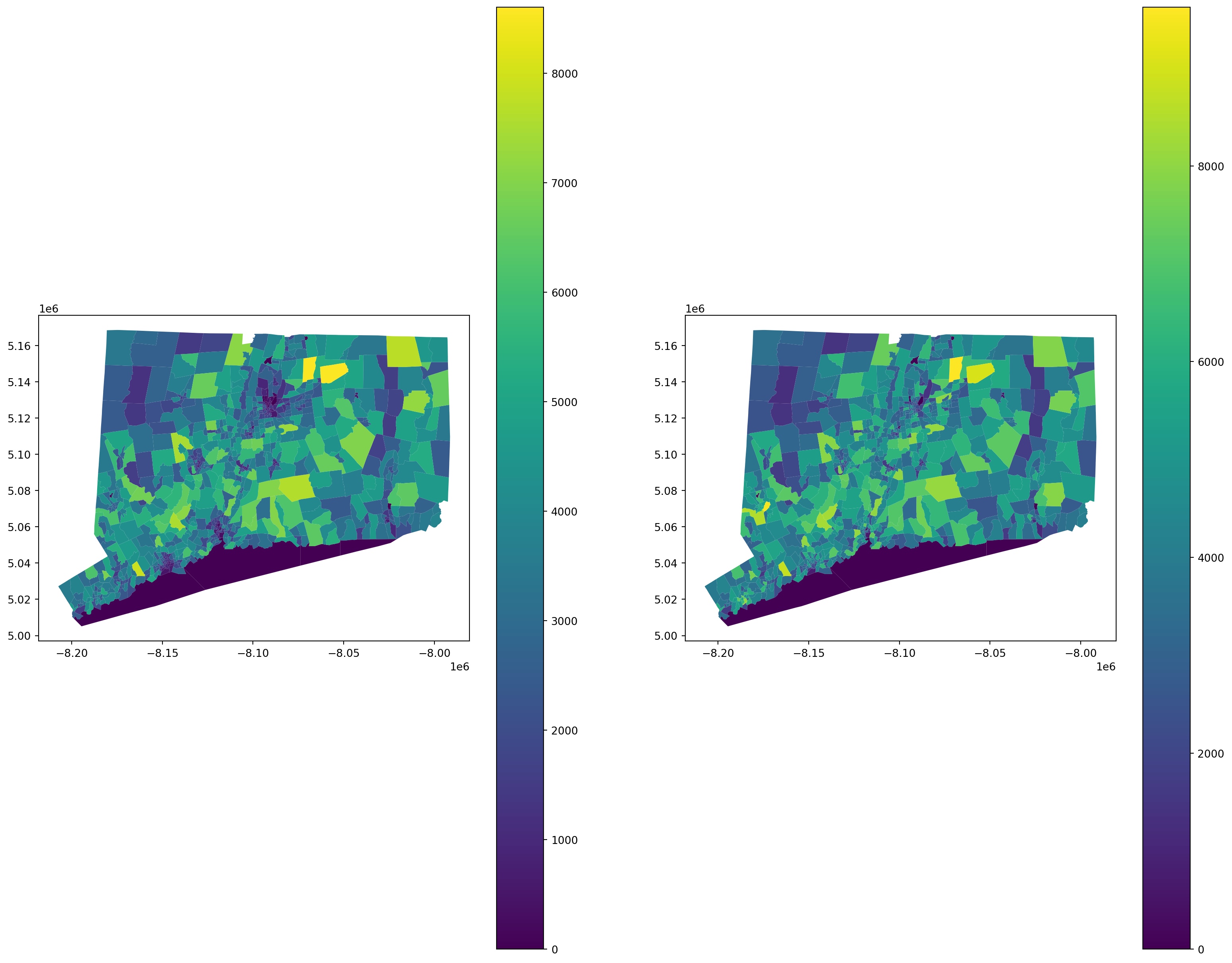
fig, (ax1,ax2) = plt.subplots(nrows=1, ncols=2, figsize=(20, 16))

ax1 = poverty_ct.plot('B17001A_001E', ax = ax1, cmap = 'viridis', legend = True)
ax2 = housing_ct.plot('B25008_001E', ax = ax2, cmap = 'viridis', legend = True)

Based on this we can visualize the numbers of individuals who are in poverty and individuals who have housing by census tract.

A further step is to run statistical analysis to see if there is any dependence and correlation between poverty and housing attainment within Connecituct.

5.5.6 References

https://cenpy-devs.github.io/cenpy/api.html https://pypi.org/project/CensusData/ https://pypi.org/project/cenpy/0.9.1/ https://geopandas.org/en/stable/getting_started/introduction.html https://data.census.gov/table/ACSDT1Y2022.B02001?t=Race+and+Ethnicity https://www.census.gov/programs-surveys/acs/technical-documentation/table-shells.2019.html#list-tab-79594641

5.6 Database Operations with SQL

5.6.1 Introduction

Today, I will be presenting on Database Operations using SQL and I will demonstrate it by using sqlite3 in Python and I will use our cleaned rodent data set. This presentation will briefly go over what Professor Haim Bar talked about during his talk and we will dive into some more advanced SQL commands.

5.6.2 What is SQL?

Structured Query Language (SQL) is a standard language for accessing and manipulating databases. It is used within relational database management systems such as MS SQL Server, MySQL, Oracle, etc… to perform CRUD operations.

5.6.2.1 CRUD

  • Create - inserting new records/values

INSERT INTO table_name VALUES (field value 1, field value 2, …)

  • Read - searching for records

SELECT field 1, field2, … FROM table_name [WHERE condition]

  • Update - modifying existing records

UPDATE table_name SET field1=value1, field2=value2, … [WHERE condition]

  • Delete - removing existing records

DELETE FROM table_name [WHERE condition]

5.6.2.2 RDBMS vs NoSQL

RDBMS

  • Basis for SQL
  • Models relationships in “Tables”
  • Rows and Columns (Record/Fields)
  • MS Access, SQL Server, MySQL
  • Two tables can be linked if they have a matching field

NoSQL

  • “Not only” SQL or Non-SQL
  • Great with large data sets
  • Key / Value Pairs
  • Does not always use SQL
  • AWS DynamoDB

5.6.3 Recap and Overview of some Basics

Key Notes from Professor Bar

5.6.3.1 Creating Tables

CREATE TABLE contacts(
    contact_id INTEGER PRIMARY KEY,
    first_name TEXT NOT NULL,
    last_name TEXT NOT NULL,
    email TEXT NOT NULL UNIQUE,
    phone TEXT NOT NULL UNIQUE
);
  • Creates a table named contacts.
  • Five fields: contact_id, first_name, last_name, email, phone
  • PRIMARY KEY: uniquely identifies each record in the table.
  • Some columns will store character data while others will store integer data.
  • NOT NULL: Columns cannot be empty.
  • UNIQUE: All values in this specific column have to be different from each other.
CREATE TABLE contact_groups (
    contact_id INTEGER PRIMARY KEY,
    group_id INTEGER PRIMARY KEY,
    PRIMARY KEY(contact_id, group_id)
    FOREIGN KEY(contact_id)
        REFERENCES contacts (contact_id)
            ON DELETE CASCADE
            ON UPDATE NO ACTION,
    FOREIGN KEY(group_id)
        REFERENCES groups (group_Id)
            ON DELETE CASCADE
            ON UPDATE NO ACTION
);
  • PRIMARY KEY() declares which variables are primary keys. We should remove the first two Primary Key declarations to have proper syntax.
  • FOREIGN KEY() declares the variable as a foreign key
    • A constraint that is used to prevent actions that would destroy links between tables.
    • A field in one table that refers to a different PRIMARY KEY in another table.
    • Table with a foreign key is a child table.
    • Prevents invalid data from being inserted into the foreign key column because it has to be a value contained in the parent table.
  • ON DELETE CASECADE: If a record in contacts is deleted, any corresponding records in contact_groups will also be deleted.
  • ON UPDATE NO ACTION: If a contact_id in contacts is updated, no action will be taken on contact_groups.
    • Can be replaced with RESTRICT.

5.6.3.2 Inserting and Searching

  • Multiple ways to insert values into a specific table.
INSERT INTO artists (name) VALUES('Bud Powell')
INSERT INTO artists (name)
VALUES
    ('Buddy Rich')
    ('Example 2')
  • Updating multiple or all rows.
SELECT employeeid, firstname, lastname, title, email FROM employees;
UPDATE employees SET lastname = 'smith' WHERE employeeid = 3;

# Multiple
UPDATE employees SET city = 'Toronto', state='ON', 
postalcode= 'M5p2n7' WHERE employeeid=4;

# All
UPDATE employees SET email = LOWER(firstname || "." || lastname || '@gmail.com';

5.6.3.3 Deleting

  • Deleting Tables/Databases
DROP TABLE addresses;
DROP DATABASE databasename;

Note: Dropping a database will result in loss of information.

  • Deleting entries given a condition
DELETE FROM table_name WHERE condition;

5.6.4 Utilizing sqlite3 in Python with Rodent Data Set

Connecting to SQLite3 Using Python

import pandas as pd
import sqlite3

# Connects to Database
conn = sqlite3.connect("presentation.db")

# Using our cleaned rodent data
data = pd.read_feather("data/rodent_2022-2023.feather")
# Creates Rodent table
data.to_sql(
            'rodent', # Name of SQL table
            conn, # sqlite3 connection
            if_exists = 'replace',
            index = False
)

# Cursor, Instance that allows you to invoke methods to execute SQL statements.
cursor = conn.cursor()

# Executing example statement to show functionality
cursor.execute("""
                SELECT *
                FROM rodent
                LIMIT 5
               """)
rows = cursor.fetchall()

# Column names
columns = [description[0] for description in cursor.description]

# Displaying the output in a table format
pd.DataFrame(rows, columns=columns)
unique_key created_date closed_date agency agency_name complaint_type descriptor location_type incident_zip incident_address ... bridge_highway_segment latitude longitude location zip_codes community_districts borough_boundaries city_council_districts police_precincts police_precinct
0 59893776 2023-12-31 23:05:41 2023-12-31 23:05:41 DOHMH Department of Health and Mental Hygiene Rodent Rat Sighting 3+ Family Apt. Building 11216 265 PUTNAM AVENUE ... None 40.683857 -73.951645 (40.683855196486164, -73.95164557951071) 17618.0 69.0 2.0 49.0 51.0 51.0
1 59887523 2023-12-31 22:19:22 2024-01-03 08:47:02 DOHMH Department of Health and Mental Hygiene Rodent Rat Sighting Commercial Building 10028 1538 THIRD AVENUE ... None 40.779243 -73.953690 (40.77924175816874, -73.95368859796383) 10099.0 23.0 4.0 1.0 11.0 11.0
2 59891998 2023-12-31 22:03:12 2023-12-31 22:03:12 DOHMH Department of Health and Mental Hygiene Rodent Rat Sighting 3+ Family Apt. Building 10458 2489 TIEBOUT AVENUE ... None 40.861694 -73.894989 (40.861693023118924, -73.89499228560491) 10936.0 6.0 5.0 22.0 29.0 29.0
3 59887520 2023-12-31 21:13:02 2024-01-03 09:33:43 DOHMH Department of Health and Mental Hygiene Rodent Mouse Sighting 3+ Family Apt. Building 11206 116 JEFFERSON STREET ... None 40.699741 -73.930733 (40.69974221739347, -73.93073474327662) 17213.0 42.0 2.0 30.0 53.0 53.0
4 59889297 2023-12-31 20:50:10 None DOHMH Department of Health and Mental Hygiene Rodent Rat Sighting 1-2 Family Dwelling 11206 114 ELLERY STREET ... None 40.698444 -73.948578 (40.69844506428295, -73.94858040356128) 17213.0 69.0 2.0 49.0 51.0 51.0

5 rows × 47 columns

5.6.5 References

  • https://www.w3schools.com/sql/
  • https://aws.amazon.com/what-is/sql/