3 Jump Start with R

This chapter gives you the minimum essentials to start using R comfortably. It assumes no prior knowledge and emphasizes good habits from the very beginning. We cover how to start and quit R, get help, understand core object types, subset objects, use basic control structures, manage your working directory, and write clean code.

Important

Rendering note. All code chunks use Quarto syntax and can be run via quarto render.

3.1 Starting and Quitting R

Start Positron, open a folder as a project, and create a new script (.R) or Quarto document (.qmd).
Run code by highlighting lines in the editor and pressing Ctrl-Enter (Win/Linux) or Cmd-Enter (Mac). The console runs one complete line at a time.
Quit with:

Code

## End your R session programmatically
q()

When asked to save the workspace, choose No. Rely on scripts for reproducibility.

3.2 Positron Interface

Positron is organized into panes and a sidebar.

Editor pane: main area for .R and .qmd files; supports tabs.
Console: interactive R prompt for quick tests.
Terminal: a shell for system commands (e.g., git, Rscript).
Files: browse, create, rename, and delete items.
Environment: lists objects in memory; clear with care.
Source control: stage, commit, and view diffs in git repos.
Command palette: Ctrl-Shift-P or Cmd-Shift-P to search commands.
Status bar: shows project folder and basic status.

Working in a project

Open a folder as the project root. Use relative paths from this root.
Keep data in data/ and scripts in R/ or src/.

Running code

Run the current line or selection with Ctrl/Cmd-Enter.
Execute a full cell in a .qmd with the Run Cell button.

Tip

Keep the Files and Console visible. Beginners benefit from constant feedback on where they are and what ran.

3.3 Getting Help

R has built‑in help for every function. Every call or command you type is calling a function.

Search the help system on a topic:

help.search("linear model")

Get the documentation of a function with known name:

?mean
help(mean)

Inspect arguments quickly for a function

Code

args(mean)

function (x, ...) 
NULL

Run examples in the documentation (man page)

example(mean)

Practice: find how sd() handles missing values.

3.4 Objects in R

Everything you store is a vector or built from vectors. Length‑one values are still vectors.

Atomic vector types (all of fixed type):

Code

## Atomic vectors (length one shown; still vectors)
num <- 3.14      ## double (numeric)
int <- 2L        ## integer
chr <- "Ann"     ## character
lgc <- TRUE      ## logical

## A longer vector (same type throughout)
v <- c(1, 2, 3)

Higher‑level structures built from vectors:

Code

## Matrix/array: same type, 2D or more
m <- matrix(1:6, nrow = 2)

## List: heterogenous elements
lst <- list(name = "Bob", age = 25, scores = c(90, 88))

## Data frame: list of equal‑length columns
## (columns can be different atomic types)
df <- data.frame(name = c("Ann", "Bob"), age = c(20, 25))

## Function: also an object
sq <- function(x) x^2

Inspect objects:

Code

## Class and structure
class(df)

[1] "data.frame"

Code

str(df)

'data.frame':   2 obs. of  2 variables:
 $ name: chr  "Ann" "Bob"
 $ age : num  20 25

Tip

Prefer str(x) for a compact view of what an object contains, its type, and its sizes.

Exercise. Create one example of each object above and check with class() and str().

3.5 Subsetting

Use bracket notation consistently.

Code

## Vectors
x <- c(2, 4, 6, 8)
x[2]             ## second element

[1] 4

Code

x[1:3]           ## slice

[1] 2 4 6

Code

x[x > 5]         ## logical filter

[1] 6 8

Code

## Matrices
m <- matrix(1:9, nrow = 3)
m[2, 3]          ## row 2, col 3

[1] 8

Code

m[, 1]           ## first column

[1] 1 2 3

Code

## Data frames
people <- data.frame(name = c("Ann", "Bob"), age = c(20, 25))
people$age       ## column by name

[1] 20 25

Code

people[1, ]      ## first row

Code

people[, "name"] ## column by string

[1] "Ann" "Bob"

3.6 Control Structures

3.6.1 If statement (missing‑value cleaning)

Code

## Replace sentinel values with NA
x <- -999
if (x == -999) {
  x <- NA
}
print(x)

[1] NA

3.6.2 For loop (column‑wise cleaning and summary)

Useful when applying a simple rule across columns.

Code

## Make a toy data frame with a sentinel value
scores <- data.frame(
  math = c(95, -999, 88, 91),
  eng  = c(87, 90, -999, 85),
  sci  = c(92, 88, 94, -999)
)

## Replace -999 with NA, then compute column means
for (col in names(scores)) {
  ## clean
  bad <- scores[[col]] == -999
  scores[[col]][bad] <- NA
  ## summarize
  m <- mean(scores[[col]], na.rm = TRUE)
  cat(col, "mean:", m, "\n")
}

math mean: 91.33333 
eng mean: 87.33333 
sci mean: 91.33333

3.6.3 While loop (simulation until tolerance met)

Stop when an estimate is precise enough.

Code

## Estimate P(X > 1.96) for N(0,1) via Monte Carlo
## Stop when stderr < 0.002
set.seed(1)
count <- 0
n <- 0
se <- Inf

while (se > 0.002) {
  ## simulate in small batches for responsiveness
  z <- rnorm(1000)
  n <- n + length(z)
  count <- count + sum(z > 1.96)
  p_hat <- count / n
  se <- sqrt(p_hat * (1 - p_hat) / n)
}

cat("p_hat:", p_hat, "n:", n, "se:", se, "\n")

p_hat: 0.0285 n: 8000 se: 0.001860368

Exercise. Write a loop that, for each numeric column in a frame, replaces -999 with NA, then reports the fraction of missing values.

Warning

Loops are fine for clarity. Later you will see vectorized and apply‑family solutions that are faster and shorter.

3.7 Workflow Basics

Code

## Working directory
getwd()                  ## where am I

[1] "/Users/junyan/work/teaching/1010-f25/1010f25"

Code

## setwd("path/to/folder")   ## set if necessary

In Positron, confirm the directory in the Files pane.
Use the console for quick tests; save work in scripts or .qmd.
Run highlighted code with Ctrl/Cmd-Enter.

Tip

Use project‑relative paths and file.path() to build paths. This keeps code portable across operating systems.

3.8 Importing Data

R can load data from text files and many other formats.

3.8.1 Base R functions

Code

## Read a CSV file (comma-separated)
cars <- read.csv("data/india.csv")

## Read a general table with custom separators
survey <- read.table("data/survey.txt", header = TRUE, sep = " ")

Arguments to know: - header = TRUE tells R the first row has column names. - sep controls the separator (“,” for CSV, ” ” for tab‑delimited).

Tip

Check the imported object with str() or head() immediately to ensure it loaded as expected.

3.8.2 Other formats

The foreign package imports legacy statistical software formats (SAS, SPSS, Stata):

Code

library(foreign)
data_spss <- read.spss("data/study.sav", to.data.frame = TRUE)
data_stata <- read.dta("data/study.dta")

More modern workflows often use the haven package (part of the tidyverse) for these formats, but foreign is available in base R distributions.

3.9 Good Style

Adopt consistent style early. Follow the tidyverse guide: https://style.tidyverse.org/

Use <- for assignment.
Place spaces around operators and after commas.
Choose meaningful names; avoid one‑letter names for data.
Begin scripts with a header block.

Code

## Your Name
## 2025-09-02
## Purpose: demonstrate basic R style
x <- 1  # inline note uses a single

Note

Comment convention. Start‑of‑line comments use at least two hashes (##). Reserve a single # for end‑of‑line notes.

3.10 Tips and Pitfalls

Case sensitivity: x and X are different.
Paths: forward slashes / work on all platforms in R.

Code

## Portable path building
file.path("data", "mtcars.csv")

[1] "data/mtcars.csv"

Numerical precision:

Code

## Floating‑point comparison
0.1 == 0.3 / 3

[1] FALSE

Code

all.equal(0.1, 0.3 / 3)

[1] TRUE

Code

## Reveal stored value with extra digits
print(0.1, digits = 20)

[1] 0.10000000000000000555

Code

sprintf("%.17f", 0.1)

[1] "0.10000000000000001"

Tip

Use all.equal() (or an absolute/relative tolerance) rather than == for real‑number comparisons.

Save code in scripts, not the workspace.
Use simple file names: letters, numbers, underscores.

3.11 Example: Hiring the Best Secretary

A manager wants to hire one secretary from among \(n\) applicants. According to some standard, the applicants can be strictly ranked from strongest to weakest, but the order in which they are interviewed is completely random. For each interview the manager must immediately decide whether to hire this person. If the applicant is hired, the process stops. Otherwise the manager moves on to the next applicant. Any rejected applicant cannot be recalled later. What rule should the manager use in order to maximize the probability that the person hired is actually the best of the \(n\) applicants?

Consider the following strategy. Choose an integer \(r < n\). The manager first interviews the first \(r\) applicants and rejects all of them. Then, starting from applicant \(r+1\), the manager hires the first applicant whose quality is better than all previous applicants. If no such applicant appears, the manager hires the last applicant.

Let \(\pi(r,n)\) be the probability that this strategy results in hiring the best applicant. It can be shown that

\[ \begin{aligned} \pi(r,n) &= \sum_{i=1}^{n} \Pr(\text{strongest in first } i-1 \text{ is in } 1,\dots,r)\, \Pr(\text{strongest at position } i) \\ &= \sum_{i=r+1}^{n} \frac{r}{i-1}\cdot \frac{1}{n}. \end{aligned} \]

The problem is to choose \(r\) to maximize \(\pi(r,n)\).

Now we estimate the probability \(\pi(r,n)\) of selecting the best candidate in the classical secretary problem using simulation in R. For each candidate number \(n\) and cutoff \(r\), we simulate the hiring process repeatedly and compute the proportion of simulations in which the selected applicant is the best (rank \(1\)).

3.11.1 One simulation of the hiring process

We represent the applicants’ true qualities as a random permutation of \(\{1,\dots,n\}\), where \(1\) is best and \(n\) is worst. With a given cutoff \(r\), we first examine the first \(r\) applicants and record the smallest (rank-best) value among them. Starting from applicant \(r+1\), we hire the first applicant whose rank is smaller than all previously observed ranks. If none is better, we hire the last applicant.

Code

secretary_once <- function(n, r) {
  # A random permutation of ranks, where 1 = best
  order <- sample.int(n)

  # Best rank seen among the first r applicants
  best_so_far <- min(order[1:r])

  # Default: hire the last applicant
  hire_index <- n

  # Look for the first applicant better than all previous ones
  if (r < n) {
    for (i in (r + 1):n) {
      if (order[i] < best_so_far) {
        hire_index <- i
        break
      }
    }
  }

  hired_rank <- order[hire_index]
  as.integer(hired_rank == 1)
}

3.11.2 Estimating \(\pi(r,n)\) through replication

We repeat the random hiring process many times and compute the average success probability.

Code

estimate_pi <- function(n, r, n_sim = 10000) {
  mean(replicate(n_sim, secretary_once(n, r)))
}

3.11.3 Searching for the optimal cutoff

For a fixed \(n\), we evaluate \(\pi(r,n)\) over \(r = 1, \dots, n-1\) and select the \(r\) that maximizes the probability of hiring the best applicant.

Code

n     <- 100
n_sim <- 2000

rs  <- 1:(n - 1)
pis <- sapply(rs, estimate_pi, n = n, n_sim = n_sim)

r_star_hat   <- rs[which.max(pis)]
max_prob_hat <- max(pis)

r_star_hat

[1] 29

Code

max_prob_hat

[1] 0.3905

We can visualize the function \(r \mapsto \pi(r,n)\):

Code

plot(rs, pis, type = "l",
     xlab = "r (cutoff)",
     ylab = "Estimated pi(r, n)",
     main = paste("Secretary Problem Simulation, n =", n))
abline(v = r_star_hat, lty = 2)
lines(rs, sapply(rs, function(r) sum((r)/((r+1):100 - 1)) / 100), col = 2, lwd = 2)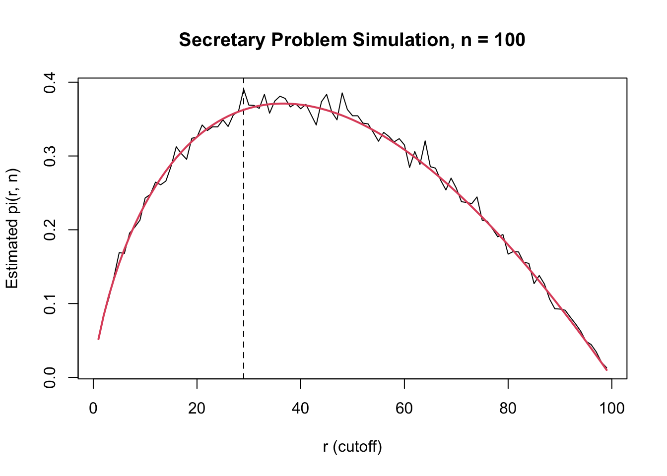

As \(n \to \infty\), \(r^* / n \to 1 / e \approx 0.368\).

3.12 Wrap‑Up Checklist

You should now be able to:

Start and quit R in Positron.
Get help with functions.
Recognize and inspect core objects with class() and str().
Subset vectors, matrices, and data frames.
Use if, for, and while in useful contexts.
Manage your working directory and paths.
Write clean, consistent code and comments.