Machine Learning (ML) is a branch of artificial intelligence that enables systems to learn from data and improve their performance over time without being explicitly programmed. At its core, machine learning algorithms aim to identify patterns in data and use those patterns to make decisions or predictions.
Machine learning can be categorized into three main types: supervised learning, unsupervised learning, and reinforcement learning. Each type differs in the data it uses and the learning tasks it performs, addressing addresses different tasks and problems. Supervised learning aims to predict outcomes based on labeled data, unsupervised learning focuses on discovering hidden patterns within the data, and reinforcement learning centers around learning optimal actions through interaction with an environment.
Let’s define some notations to introduce them:
\(X\): A set of feature vectors representing the input data. Each element \(X_i\) corresponds to a set of features or attributes that describe an instance of data.
\(Y\): A set of labels or rewards associated with outcomes. In supervised learning, \(Y\) is used to evaluate the correctness of the model’s predictions. In reinforcement learning, \(Y\) represents the rewards that guide the learning process.
\(A\): A set of possible actions in a given context. In reinforcement learning, actions \(A\) represent choices that can be made in response to a given situation, with the goal of maximizing a reward.
9.1.1 Supervised Learning
Supervised learning is the most widely used type of machine learning. In supervised learning, we have both feature vectors \(X\) and their corresponding labels \(Y\). The objective is to train a model that can predict \(Y\) based on \(X\). This model is trained on labeled examples, where the correct outcome is known, and it adjusts its internal parameters to minimize the error in its predictions, which occurs as part of the cross-validation process.
Key tasks in supervised learning include:
Classification: Assigning data points to predefined categories or classes.
Regression: Predicting a continuous value based on input data.
In supervised learning, the data consists of both feature vectors \(X\) and labels \(Y\), namely, \((X, Y)\).
9.1.2 Unsupervised Learning
Unsupervised learning involves learning patterns from data without any associated labels or outcomes. The objective is to explore and identify hidden structures in the feature vectors \(X\). Since there are no ground-truth labels \(Y\) to guide the learning process, the algorithm must discover patterns on its own. This is particularly useful when subject matter experts are unsure of common properties within a data set.
Common tasks in unsupervised learning include:
Clustering: Grouping similar data points together based on certain features.
Dimension Reduction: Simplifying the input data by reducing the number of features while preserving essential patterns.
In unsupervised learning, the data consists solely of feature vectors \(X\).
9.1.3 Reinforcement Learning
Reinforcement learning involves learning how to make a sequence of decisions to maximize a cumulative reward. Unlike supervised learning, where the model learns from a static dataset of labeled examples, reinforcement learning involves an agent that interacts with an environment by taking actions \(A\), receiving feedback in the form of rewards \(Y\), and learning over time which actions lead to the highest cumulative reward.
The process in reinforcement learning involves:
States: The context or environment the agent is in, represented by feature vectors \(X\).
Actions: The set of possible choices the agent can make in response to the current state, denoted as \(A\).
Rewards: Feedback the agent receives after taking an action, which guides the learning process.
In reinforcement learning, the data consists of feature vectors \(X\), actions \(A\), and rewards \(Y\), namely, \((X, A, Y)\).
9.2 Bias-Variance Tradeoff
The variance-bias trade-off is a core concept in machine learning that explains the relationship between the complexity of a model, its performance on training data, and its ability to generalize to unseen data. It applies to both supervised and unsupervised learning, though it manifests differently in each.
9.2.1 Bias
Bias refers to the error introduced by approximating a complex real-world problem with a simplified model. A model with high bias makes strong assumptions about the data, leading to oversimplified patterns and poor performance on both the training data and new data. High bias results in underfitting, where the model fails to capture important trends in the data.
Example (Supervised): In supervised learning, using a linear regression model to fit data that has a nonlinear relationship results in high bias because the model cannot capture the complexity of the data.
Example (Unsupervised): In clustering (an unsupervised task), setting the number of clusters too low (e.g., forcing data into two clusters when more exist) leads to high bias, as the model oversimplifies the underlying structure.
9.2.2 Variance
Variance refers to the model’s sensitivity to small changes in the training data. A model with high variance will adapt closely to the training data, potentially capturing noise or fluctuations that are not representative of the general data distribution. High variance leads to overfitting, where the model performs well on training data but poorly on new, unseen data.
Example (Supervised): A decision tree with many branches can exhibit high variance. The model perfectly fits the training data but may perform poorly on test data because it overfits to specific idiosyncrasies in the training set.
Example (Unsupervised): In clustering, setting the number of clusters too high or fitting overly flexible cluster shapes (e.g., in Gaussian Mixture Models) can lead to overfitting, where the model captures noise and splits data unnecessarily.
9.2.3 The Trade-Off
The bias-variance trade-off reflects the tension between bias and variance. As model complexity increases:
Bias decreases: The model becomes more flexible and can capture more details of the data.
Variance increases: The model becomes more sensitive to the particular training data, potentially capturing noise.
Conversely, a simpler model will:
Have high bias: It may not capture all relevant patterns in the data.
Have low variance: It will be less sensitive to fluctuations in the data and is more likely to generalize well to unseen data.
9.2.4 Bias-Variance in Supervised Learning
In supervised learning, the goal is to strike the right balance between bias and variance to minimize prediction error. This balance is critical for developing models that generalize well to new data. The total error of a model can be decomposed into:
Bias: The error from using a model that is too simple.
Variance: The error from using a model that is too complex and overfits the training data.
Irreducible Error: This is the noise inherent in the data itself, which cannot be eliminated no matter how well the model is tuned.
9.2.5 Bias-Variance in Unsupervised Learning
In unsupervised learning, the bias-variance trade-off is less formally defined but still relevant. For example:
In clustering, choosing the wrong number of clusters can lead to either high bias (too few clusters, oversimplifying the data) or high variance (too many clusters, overfitting the data).
In dimensionality reduction, keeping too few components in Principal Component Analysis (PCA) increases bias by losing important information, while keeping too many components retains noise, increasing variance.
In unsupervised learning, balancing bias and variance typically involves tuning hyperparameters (e.g., number of clusters, number of components) to find the right complexity level.
9.2.6 Striking the Right Balance
To strike the balance between bias and variance in both supervised and unsupervised learning, techniques such as regularization, early stopping, cross-validation, and hyperparameter tuning are essential. These techniques help ensure the model is complex enough to capture patterns in the data but not so complex that it overfits to noise or irrelevant details.
9.3 Crossvalidation
Cross-validation is a technique used to evaluate machine learning models and tune hyperparameters by splitting the dataset into multiple subsets. This approach helps to avoid overfitting and provides a better estimate of the model’s performance on unseen data. Cross-validation is especially useful for managing the bias-variance trade-off by allowing you to test how well the model generalizes without relying on a single train-test split.
9.3.1 K-Fold Cross-Validation
The most commonly used method is \(k\)-fold cross-validation:
Split the data: The dataset is divided into \(k\) equally-sized folds (subsets).
Train on \(k - 1\) folds: The model is trained on \(k - 1\) folds, leaving one fold as a test set.
Test on the remaining fold: The model’s performance is evaluated on the fold that was left out.
Repeat: This process is repeated \(k\) times, with each fold used once as the test set.
Average performance: The final cross-validation score is the average performance across all \(k\) iterations.
By averaging the results across multiple test sets, cross-validation provides a more robust estimate of model performance and helps avoid overfitting or underfitting to any particular training-test split.
Leave-One-Out Cross-Validation (LOOCV) takes each observation as one fold. The dataset is split into \(n\) subsets (where \(n\) is the sample size), with each sample acting as a test set once. While this method provides the most exhaustive evaluation, it can be computationally expensive for large datasets.
9.3.2 Benefits of Cross-Validation
Prevents overfitting: By testing the model on multiple subsets of data, cross-validation helps to identify if the model is too complex and overfits to the training data.
Prevents underfitting: If the model performs poorly across all folds, it may indicate that the model is too simple (high bias).
Better estimation: Cross-validation gives a better estimate of how the model will perform on unseen data compared to a single train-test split.
9.3.3 Cross-Validation in Unsupervised Learning
While cross-validation is most commonly used in supervised learning, it can also be applied to unsupervised learning through:
Stability testing: Running unsupervised algorithms (e.g., clustering) on different data splits and measuring the stability of the results (e.g., using the silhouette score).
Internal validation metrics: In clustering, internal metrics like the silhouette score or Davies-Bouldin index can be used to evaluate the quality of clustering across different data splits.
The bias-variance trade-off is a universal problem in machine learning, affecting both supervised and unsupervised models. Cross-validation is a powerful tool for controlling this trade-off by providing a reliable estimate of model performance and helping to fine-tune model complexity. By balancing bias and variance through careful model selection, regularization, and cross-validation, you can develop models that generalize well to unseen data without overfitting or underfitting.
9.3.4 A Curve-Fitting with Splines: An Example
Overfitting occurs when a model becomes overly complex and starts to capture not just the underlying patterns in the data but also the noise or random fluctuations. This can lead to poor generalization to new, unseen data. A clear sign of overfitting is when a model performs very well on the training data but performs poorly on test data, as it fails to generalize beyond the data it was trained on.
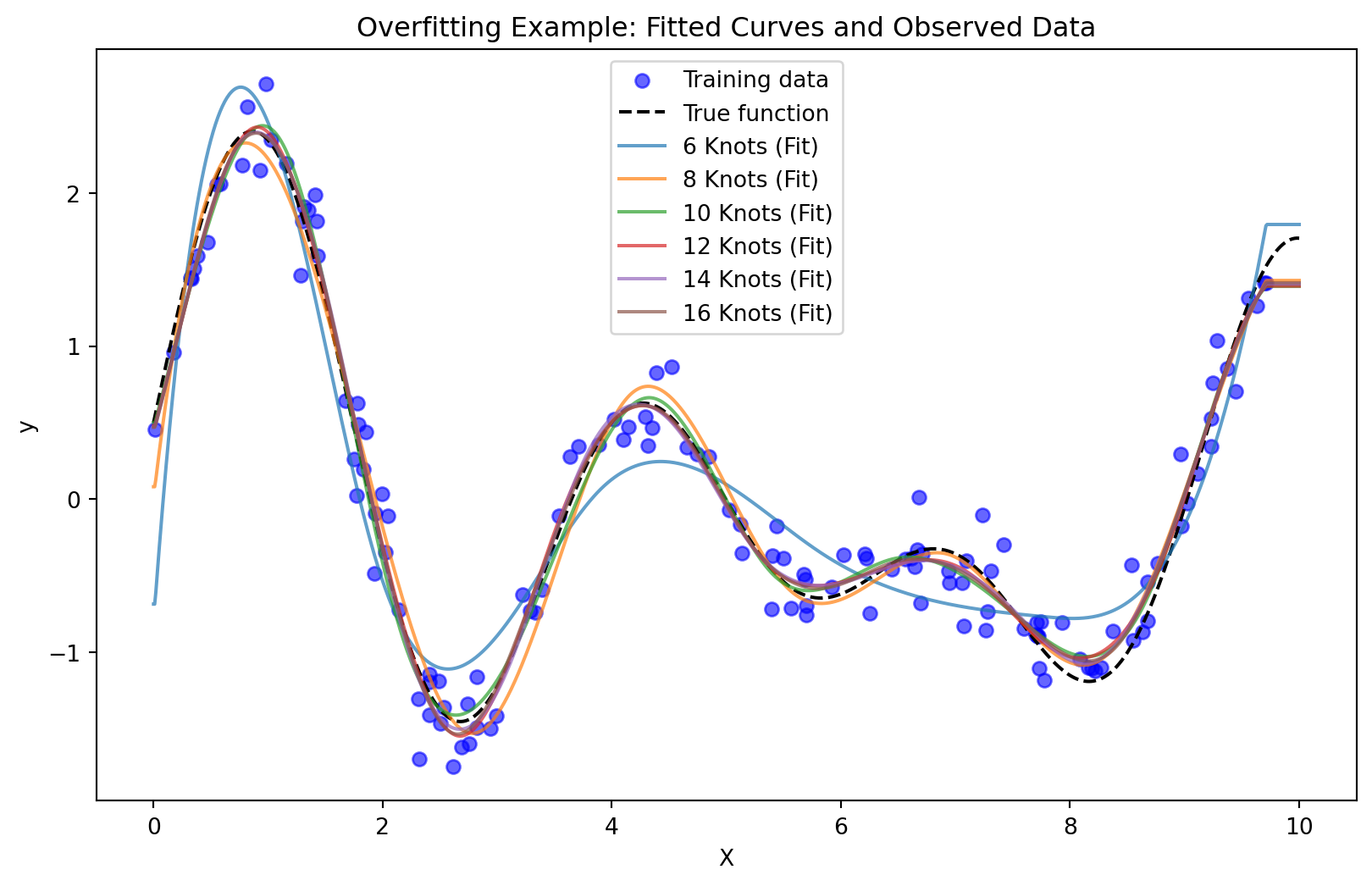
In this example, we illustrate overfitting using cubic spline regression with different numbers of knots. Splines are a flexible tool that allow for piecewise polynomial regression, with knots defining where the pieces of the polynomial meet. The more knots we use, the more flexible the model becomes, which can potentially lead to overfitting.
import numpy as npimport matplotlib.pyplot as pltfrom sklearn.model_selection import train_test_splitfrom sklearn.preprocessing import SplineTransformerfrom sklearn.linear_model import LinearRegressionfrom sklearn.pipeline import make_pipelinefrom sklearn.metrics import mean_squared_errordef true_function(X):return np.sin(1.5* X) +0.5* np.cos(0.5* X) + np.sin(2* X)# Generate synthetic data using the more complex true functionX = np.sort(np.random.rand(200) *10).reshape(-1, 1)y = true_function(X).ravel() + np.random.normal(0, 0.2, X.shape[0])# Split data into training and test setsX_train, X_test, y_train, y_test = train_test_split(X, y, test_size=0.3, random_state=42)# Function to explore overfitting by plotting both errors and fitted curvesdef overfitting_example_with_fitted_curves(X_train, y_train, X_test, y_test, knots_list): train_errors = [] test_errors = []# Generate fine grid for plotting the true curve and fitted models X_line = np.linspace(0, 10, 1000).reshape(-1, 1) y_true = true_function(X_line)# Plot the true function and observed data plt.figure(figsize=(10, 6)) plt.scatter(X_train, y_train, color='blue', label='Training data', alpha=0.6) plt.plot(X_line, y_true, label='True function', color='black', linestyle='--')for n_knots in knots_list:# Create a spline model with fixed degree = 3 (cubic) and varying knots spline = SplineTransformer(degree=3, n_knots=n_knots, include_bias=False) model = make_pipeline(spline, LinearRegression())# Fit the model to training data model.fit(X_train, y_train)# Predict on training and test data y_pred_train = model.predict(X_train) y_pred_test = model.predict(X_test) y_pred = model.predict(X_line)# Calculate training and test errors (mean squared error) train_errors.append(mean_squared_error(y_train, y_pred_train)) test_errors.append(mean_squared_error(y_test, y_pred_test))# Plot the fitted curve plt.plot(X_line, y_pred, label=f'{n_knots} Knots (Fit)', alpha=0.7)print(train_errors, test_errors) plt.title('Overfitting Example: Fitted Curves and Observed Data') plt.xlabel('X') plt.ylabel('y') plt.legend() plt.show()# Plot training and test error separately plt.figure(figsize=(10, 6)) plt.plot(knots_list, train_errors, label='Training Error', marker='o', color='blue') plt.plot(knots_list, test_errors, label='Test Error', marker='o', color='red') plt.title('Training vs. Test Error with Varying Knots') plt.xlabel('Number of Knots') plt.ylabel('Mean Squared Error') plt.legend() plt.show()# Explore overfitting by varying the number of knots and overlaying the fitted curvesknots_list = [6, 8, 10, 12, 14, 16]overfitting_example_with_fitted_curves(X_train, y_train, X_test, y_test, knots_list)
In the first plot, we fit cubic splines with 2, 4, 6, 8, 10, and 12 knots to the data. As the number of knots increases, the model becomes more flexible and better able to fit the training data. With only 2 knots, the model is quite smooth and underfits the data, capturing only broad trends but missing the detailed structure of the true underlying function. With 4 or 6 knots, the model begins to capture more of the data’s structure, balancing the bias-variance trade-off effectively. However, as we increase the number of knots to 10 and 12, the model becomes too flexible. It starts to fit the noise in the training data, producing a curve that adheres too closely to the data points. This is a classic case of overfitting: the model fits the training data very well, but it no longer generalizes to new data.
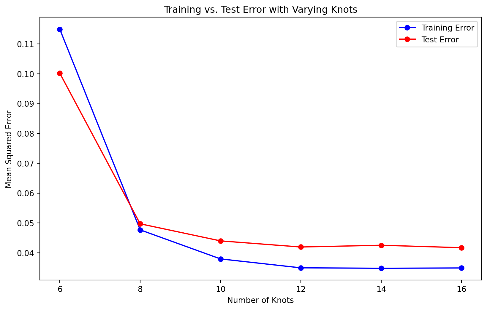
In the second plot, we observe the training error and test error as the number of knots increases. As expected, the training error consistently decreases as the number of knots increases, since a more complex model can fit the training data better. However, the test error tells a different story. Initially, the test error decreases as the model becomes more flexible, indicating that the model is learning meaningful patterns from the data. But after a certain point, the test error begins to increase, signaling overfitting.
This is a key insight into the bias-variance trade-off. While adding more complexity (in this case, more knots) reduces bias and improves fit on the training data, it also increases variance, making the model more sensitive to fluctuations and noise in the data. This results in worse performance on test data, as the model becomes too specialized to the training set.
The example clearly demonstrates how overfitting can occur when the model becomes too complex. In practice, it’s important to find a balance between underfitting (high bias) and overfitting (high variance). Techniques such as cross-validation, regularization, or limiting model complexity (e.g., setting a reasonable number of knots in spline regression) can help manage this trade-off and produce models that generalize well to unseen data.
By tuning the number of knots or other model parameters, we can achieve a model that strikes the right balance, capturing the true patterns in the data without fitting the noise.