from shapely.geometry import LineString, Point, Polygon
import geopandas as gpd
# point example
point = Point(0.5, 0.5)
gdf1 = gpd.GeoDataFrame(geometry=[point])
# line example
line = LineString([(0, 0), (1, 1)])
gdf2 = gpd.GeoDataFrame(geometry=[line])
# polygon example
polygon = Polygon([(0, 0), (0, 1), (1, 1), (1, 0), (0, 0)])
gdf3 = gpd.GeoDataFrame(geometry=[polygon])6 Geospatial Data
6.1 Handling Spatial Data with GeoPandas (by Kaitlyn Bedard)
GeoPandas is a python library created as an extension of pandas to offer support for geographic data. Like pandas, GeoPandas has a series type and a dataframe type: GeoSeries and GeoDataFrame. It allows users to do work that would otherwise need a GIS database. Note that since GeoPandas is an extension of Pandas, it inherits all its attributes and methods. Please review the pandas presentations for information on these tools, if needed.
6.1.1 Installation
You can install GeoPandas using the below commands in terminal. The documentation recommends the first method.
conda install -c conda-forge geopandas
conda install geopandas
pip install geopandas
6.1.2 Basic Concepts
The GeoPandas GeoDataFrame is essentially a pandas dataframe that supports typical data, however, it also supports geometries. Though the dataframe can have multiple geometry columns, there is one “active” column on which all operations are applied to.
The types of geometries are:
- Points: coordinates
- Lines: set of two coordinates
- Polygons: list of coordinate tuples, first and last must be the same (closed shape)
These geometries are often represented by shapely.geometry objects. Note, we can also have multi-points, multi-lines, and multi-polygons. Below are examples of creating these geometries using shapely. Each GeoSeries has a specified CRS (Coordinate Reference System) that stores information about the data.
The following are some examples of basic attributes of a GeoSeries:
length: returns the length of a line
gdf2.length0 1.414214
dtype: float64area: returns the area of the shape
gdf3.area0 1.0
dtype: float64bounds: gives the bounds of each row in a geometry columntotal_bounds: gives the total bounds of a geometry seriesgeom_type: gives the geometry type
gdf3.geom_type0 Polygon
dtype: objectis_valid: returns True for valid geometries and False otherwise
Below are some examples of basic methods that can be applied to a GeoSeries:
distance(): returns the (minimum) distance of each row of a geometry to a specified paramater- parameter
other: can be a single geometry, or an entire geometry series - parameter
align: True if you want to align GeoSeries by index, false otherwise
- parameter
gdf2.distance(Point((1,0)))0 0.707107
dtype: float64centroid: returns a new GeoSeries with the centers of each row in the geometry
gdf3.centroid0 POINT (0.50000 0.50000)
dtype: geometryBelow are examples of some relationship tests that can be applied to a GeoSeries:
contains(): returns true if shape contains a specifiedother- parameter
other: can be a single geometry, or an entire geometry series - parameter
align: True if you want to align GeoSeries by index, false otherwise
- parameter
gdf3.contains(gdf1)0 True
dtype: boolintersects(): returns true if shape intersects a specifiedother- parameter
other: can be a single geometry, or an entire geometry series - parameter
align: True if you want to align GeoSeries by index, false otherwise
- parameter
gdf2.intersects(gdf3)0 True
dtype: bool6.1.3 Reading Files
If you have a file that contains data and geometry information, you can read it directly with geopandas using the geopandas.read_file() command. Examples of these files are GeoPackage, GeoJSON, Shapefile. However, we can convert other types of files to a GeoDataFrame. For example, we can transform the NYC crash data. The below code creates a point geometry. The points are the coordinates of the crashes.
# Reading csv file
import pandas as pd
import numpy as np
# Shapely for converting latitude/longtitude to geometry
from shapely.geometry import Point
# To create GeodataFrame
import geopandas as gpd
jan23 = pd.read_csv('data/nyc_crashes_202301_cleaned.csv')
# creating geometry using shapely (removing empty points)
geometry = [Point(xy) for xy in zip(jan23["LONGITUDE"], \
jan23["LATITUDE"]) if not Point(xy).is_empty]
# creating geometry column to be used by geopandas
geometry2 = gpd.points_from_xy(jan23["LONGITUDE"], jan23["LATITUDE"])
# coordinate reference system (epsg:4326 implies geographic coordinates)
crs = {'init': 'epsg:4326'}
# create Geographic data frame (removing rows with missing coordinates)
jan23_gdf = gpd.GeoDataFrame(jan23.loc[~pd.isna(\
jan23["LATITUDE"]) & ~pd.isna(\
jan23["LONGITUDE"])],crs=crs, geometry=geometry)
jan23_gdf.head()/usr/local/lib/python3.11/site-packages/pyproj/crs/crs.py:141: FutureWarning: '+init=<authority>:<code>' syntax is deprecated. '<authority>:<code>' is the preferred initialization method. When making the change, be mindful of axis order changes: https://pyproj4.github.io/pyproj/stable/gotchas.html#axis-order-changes-in-proj-6
in_crs_string = _prepare_from_proj_string(in_crs_string)| CRASH DATE | CRASH TIME | BOROUGH | ZIP CODE | LATITUDE | LONGITUDE | LOCATION | ON STREET NAME | CROSS STREET NAME | OFF STREET NAME | ... | Unnamed: 31 | Unnamed: 32 | Unnamed: 33 | Unnamed: 34 | Unnamed: 35 | Unnamed: 36 | Unnamed: 37 | Unnamed: 38 | Unnamed: 39 | geometry | |
|---|---|---|---|---|---|---|---|---|---|---|---|---|---|---|---|---|---|---|---|---|---|
| 0 | 1/1/23 | 14:38 | BROOKLYN | 11211.0 | 40.719094 | -73.946108 | (40.7190938,-73.9461082) | BROOKLYN QUEENS EXPRESSWAY RAMP | NaN | NaN | ... | NaN | NaN | NaN | NaN | NaN | NaN | NaN | NaN | NaN | POINT (-73.94611 40.71909) |
| 1 | 1/1/23 | 8:04 | QUEENS | 11430.0 | 40.659508 | -73.773687 | (40.6595077,-73.7736867) | NASSAU EXPRESSWAY | NaN | NaN | ... | NaN | NaN | NaN | NaN | NaN | NaN | NaN | NaN | NaN | POINT (-73.77369 40.65951) |
| 2 | 1/1/23 | 18:05 | MANHATTAN | 10011.0 | 40.742454 | -74.008686 | (40.7424543,-74.008686) | 10 AVENUE | 11 AVENUE | NaN | ... | NaN | NaN | NaN | NaN | NaN | NaN | NaN | NaN | NaN | POINT (-74.00869 40.74245) |
| 3 | 1/1/23 | 23:45 | QUEENS | 11103.0 | 40.769737 | -73.912440 | (40.769737, -73.91244) | ASTORIA BOULEVARD | 37 STREET | NaN | ... | NaN | NaN | NaN | NaN | NaN | NaN | NaN | NaN | NaN | POINT (-73.91244 40.76974) |
| 4 | 1/1/23 | 4:50 | BRONX | 10462.0 | 40.830555 | -73.850720 | (40.830555, -73.85072) | CASTLE HILL AVENUE | EAST 177 STREET | NaN | ... | NaN | NaN | NaN | NaN | NaN | NaN | NaN | NaN | NaN | POINT (-73.85072 40.83055) |
5 rows × 41 columns
6.1.4 Plotting
We can easily plot our data now that has been transformed to a geometric data frame.
# Basic Plot
jan23_gdf.plot()
# Color the plot by borough
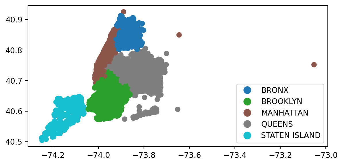
jan23_gdf.plot(column = 'BOROUGH',legend=True)
# Color the plot by number persons injuried
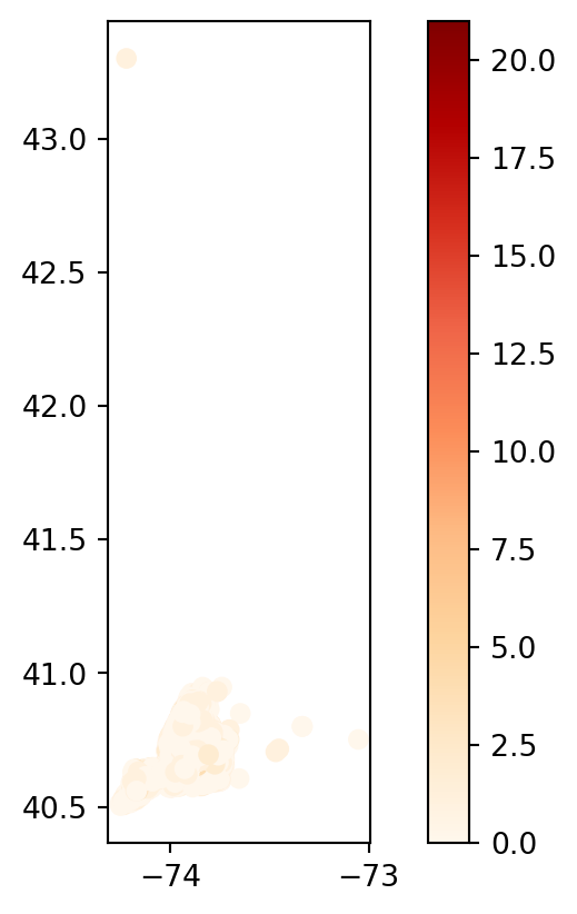
jan23_gdf.plot(column = 'NUMBER OF PERSONS INJURED',legend=True, \
cmap= "OrRd")
# Plotting missing information
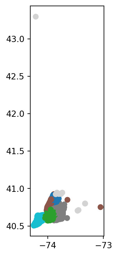
jan23_gdf.plot(column='BOROUGH', missing_kwds={'color': 'lightgrey'})<AxesSubplot: >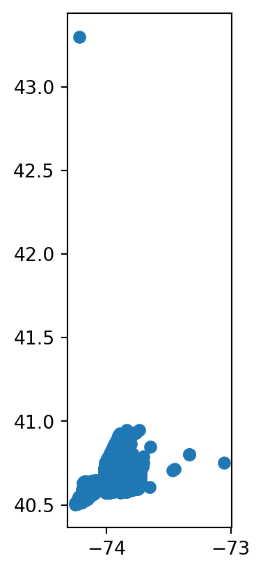
6.1.5 Interactive Maps
We can also easily create an interactive plot, using the .explore() method.
# interactive map of just the latitude and longitude points
jan23_gdf.explore()Make this Notebook Trusted to load map: File -> Trust Notebook
# interactive map where points are colored by borough
jan23_gdf.explore(column='BOROUGH',legend=True)Make this Notebook Trusted to load map: File -> Trust Notebook
# interative map that plots the crashes where 1+ persons are killed
jan23_gdf_edit = jan23_gdf.copy()
jan23_gdf_edit = jan23_gdf[jan23_gdf["NUMBER OF PERSONS KILLED"] > 0]
jan23_gdf_edit.explore(column='NUMBER OF PERSONS KILLED', \
style_kwds={'radius': 7})Make this Notebook Trusted to load map: File -> Trust Notebook
6.1.6 Setting and Changing Projections
Earlier, we showed how to set a CRS using crs = {'init': 'epsg:4326'}. However, the CRS can also be set using the .set_crs function on GeoDataFrame that does not yet have a defined CRS. Going back to our first example, gdf1, we can set the CRS as follows.
gdf1 = gdf1.set_crs("EPSG:4326")
gdf1.plot()<AxesSubplot: >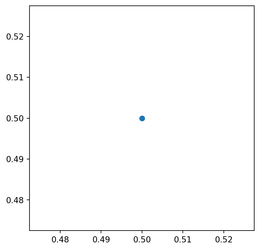
We can also change the CRS of a geometry using the .to_crs() function. Some options are:
EPSG:3395 - World Mercator system
ESPG:4326 - Standard Coordinates
EPSG:2163 - NAD83, a system for the US and Canada
Note that 4326 is the most common.
6.1.7 Merging Data and Demonstrations
The below code imports the NYC borough and zip code level spatial data.
import geopandas as gpd
# import NYC Borough Data
boros = gpd.read_file("data/nyc_boroughs.geojson")
boros.set_crs("EPSG:4326")
boros.head()| boro_code | boro_name | shape_area | shape_leng | geometry | |
|---|---|---|---|---|---|
| 0 | 5 | Staten Island | 1623620725.06 | 325917.353702 | MULTIPOLYGON (((-74.05051 40.56642, -74.05047 ... |
| 1 | 2 | Bronx | 1187182350.92 | 463176.004334 | MULTIPOLYGON (((-73.89681 40.79581, -73.89694 ... |
| 2 | 3 | Brooklyn | 1934229471.99 | 728263.543413 | MULTIPOLYGON (((-73.86327 40.58388, -73.86381 ... |
| 3 | 1 | Manhattan | 636520830.696 | 357564.317228 | MULTIPOLYGON (((-74.01093 40.68449, -74.01193 ... |
| 4 | 4 | Queens | 3041418543.49 | 888199.780587 | MULTIPOLYGON (((-73.82645 40.59053, -73.82642 ... |
# import NYC Zip Code Data
zipcodes = gpd.read_file("data/nyc_zipcodes.geojson")
zipcodes.set_crs("EPSG:4326")
zipcodes.head()| ZIPCODE | BLDGZIP | PO_NAME | POPULATION | AREA | STATE | COUNTY | ST_FIPS | CTY_FIPS | URL | SHAPE_AREA | SHAPE_LEN | geometry | |
|---|---|---|---|---|---|---|---|---|---|---|---|---|---|
| 0 | 11436 | 0 | Jamaica | 18681.0 | 2.269930e+07 | NY | Queens | 36 | 081 | http://www.usps.com/ | 0.0 | 0.0 | POLYGON ((-73.80585 40.68291, -73.80569 40.682... |
| 1 | 11213 | 0 | Brooklyn | 62426.0 | 2.963100e+07 | NY | Kings | 36 | 047 | http://www.usps.com/ | 0.0 | 0.0 | POLYGON ((-73.93740 40.67973, -73.93487 40.679... |
| 2 | 11212 | 0 | Brooklyn | 83866.0 | 4.197210e+07 | NY | Kings | 36 | 047 | http://www.usps.com/ | 0.0 | 0.0 | POLYGON ((-73.90294 40.67084, -73.90223 40.668... |
| 3 | 11225 | 0 | Brooklyn | 56527.0 | 2.369863e+07 | NY | Kings | 36 | 047 | http://www.usps.com/ | 0.0 | 0.0 | POLYGON ((-73.95797 40.67066, -73.95576 40.670... |
| 4 | 11218 | 0 | Brooklyn | 72280.0 | 3.686880e+07 | NY | Kings | 36 | 047 | http://www.usps.com/ | 0.0 | 0.0 | POLYGON ((-73.97208 40.65060, -73.97192 40.650... |
I will demonstrate some more tools using the NYC Borough data, NYC Zip Code data, NYC Crash Data, and the merged data sets.
We can plot the borough data based on the number of people killed, for example. First, compute the average number of deaths per borough. Then merge the averages into the borough data frame, and plot accordingly.
# change input to match
boros['boro_name'] = boros['boro_name'].apply(lambda x: x.upper())
# change name of column to match
jan23_gdf = jan23_gdf.rename(columns={"BOROUGH":"boro_name"})
# Compute the average number of deaths per borough
avg_deaths_per_boro = jan23_gdf.groupby('boro_name')['NUMBER OF PERSONS KILLED'].mean()
# Merge the average deaths per borough back into the borough GeoDataFrame
boros = boros.merge(avg_deaths_per_boro, on='boro_name', suffixes=('', '_mean'))
boros.head()| boro_code | boro_name | shape_area | shape_leng | geometry | NUMBER OF PERSONS KILLED | |
|---|---|---|---|---|---|---|
| 0 | 5 | STATEN ISLAND | 1623620725.06 | 325917.353702 | MULTIPOLYGON (((-74.05051 40.56642, -74.05047 ... | 0.007812 |
| 1 | 2 | BRONX | 1187182350.92 | 463176.004334 | MULTIPOLYGON (((-73.89681 40.79581, -73.89694 ... | 0.000848 |
| 2 | 3 | BROOKLYN | 1934229471.99 | 728263.543413 | MULTIPOLYGON (((-73.86327 40.58388, -73.86381 ... | 0.001676 |
| 3 | 1 | MANHATTAN | 636520830.696 | 357564.317228 | MULTIPOLYGON (((-74.01093 40.68449, -74.01193 ... | 0.003101 |
| 4 | 4 | QUEENS | 3041418543.49 | 888199.780587 | MULTIPOLYGON (((-73.82645 40.59053, -73.82642 ... | 0.002525 |
# plot
boros.plot(column = "NUMBER OF PERSONS KILLED", legend = True)<AxesSubplot: >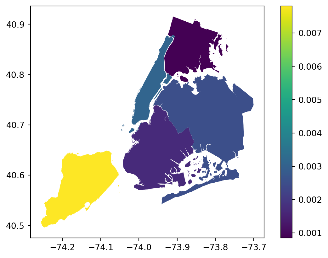
We can follow this same process to plot the average number of injuries on the zip code level.
# format changes
jan23_gdf = jan23_gdf.rename(columns={"ZIP CODE":"ZIPCODE"})
jan23_gdf["ZIPCODE"] = jan23_gdf["ZIPCODE"].replace(np.nan, 0)
jan23_gdf["ZIPCODE"] = jan23_gdf["ZIPCODE"].astype(int)
jan23_gdf["ZIPCODE"] = jan23_gdf["ZIPCODE"].astype(str)
jan23_gdf["ZIPCODE"] = jan23_gdf["ZIPCODE"].replace('0', np.nan)
# Compute the average number of injuries per zipcode
avg_injuries_per_zip = jan23_gdf.groupby('ZIPCODE')['NUMBER OF PERSONS INJURED'].mean()
# Merge the average injuries per zip back into the zipcodes GeoDataFrame
zipcodes = zipcodes.merge(avg_injuries_per_zip, on='ZIPCODE', suffixes=('', '_mean'))
zipcodes.head()| ZIPCODE | BLDGZIP | PO_NAME | POPULATION | AREA | STATE | COUNTY | ST_FIPS | CTY_FIPS | URL | SHAPE_AREA | SHAPE_LEN | geometry | NUMBER OF PERSONS INJURED | |
|---|---|---|---|---|---|---|---|---|---|---|---|---|---|---|
| 0 | 11436 | 0 | Jamaica | 18681.0 | 2.269930e+07 | NY | Queens | 36 | 081 | http://www.usps.com/ | 0.0 | 0.0 | POLYGON ((-73.80585 40.68291, -73.80569 40.682... | 0.535714 |
| 1 | 11213 | 0 | Brooklyn | 62426.0 | 2.963100e+07 | NY | Kings | 36 | 047 | http://www.usps.com/ | 0.0 | 0.0 | POLYGON ((-73.93740 40.67973, -73.93487 40.679... | 0.573034 |
| 2 | 11212 | 0 | Brooklyn | 83866.0 | 4.197210e+07 | NY | Kings | 36 | 047 | http://www.usps.com/ | 0.0 | 0.0 | POLYGON ((-73.90294 40.67084, -73.90223 40.668... | 0.627907 |
| 3 | 11225 | 0 | Brooklyn | 56527.0 | 2.369863e+07 | NY | Kings | 36 | 047 | http://www.usps.com/ | 0.0 | 0.0 | POLYGON ((-73.95797 40.67066, -73.95576 40.670... | 0.970588 |
| 4 | 11218 | 0 | Brooklyn | 72280.0 | 3.686880e+07 | NY | Kings | 36 | 047 | http://www.usps.com/ | 0.0 | 0.0 | POLYGON ((-73.97208 40.65060, -73.97192 40.650... | 0.660377 |
# plot
zipcodes.explore(column = "NUMBER OF PERSONS INJURED", legend = True)Make this Notebook Trusted to load map: File -> Trust Notebook
We can also plot the number of crashes by zip code (or borough) as well. See the below code:
# count the number of crashes per zipcode
crash_count_by_zipcode = jan23_gdf.groupby('ZIPCODE')['CRASH DATE'].count().reset_index()
# merge the count with the zipcodes data frame
zipcodes_with_crash_count = zipcodes.merge(crash_count_by_zipcode, on='ZIPCODE')
# plot
zipcodes_with_crash_count.plot(column='CRASH DATE', cmap='OrRd', legend=True)<AxesSubplot: >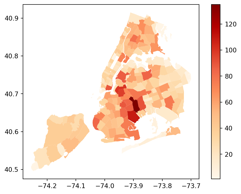
6.1.8 Resources
For more information see the following:
- GeoPandas Documentation
- NYC Borough Data
- NYC Zip Code Data
6.2 Plot on Maps with gmplot (by Luke Noel)
6.2.1 Introduction
Python package gmplot allows plotting data on Google Maps using geographical coordinates. It has a matplotlib-like interface where we can save an HTML file of the map output in our local files.
6.2.2 Installation
Before we can use this package, we need to install it using our command line.
pip install gmplot6.2.3 Importing the Package
We can now import gmplot and use it in our python code
import gmplot6.2.4 API Key
You can use the gmplot package without a Google API key, but your map output will be greyed out and have watermarks over it. To remove these you need to create your own Google Maps API key and call it in your python code. You can get started by using this link: https://developers.google.com/maps/documentation/embed/get-api-key.
Here is an example of what a map looks like without using your API key:
For the following code to work with an API key, you need to set the variable apikey with your own key.
apikey = 'please put your key in this quote'These Google Map outputs are stored as HTML files that you open and interact with in your browser. However, for the sake of this presentation, I have screenshotted some of these plots and saved them as png files to show some pictures in this notebook.
6.2.5 GoogleMapPlotter
The main function in gmplot is GoogleMapPlotter, which, as it says in the name, is a plotter that draws on a Google Map. Use this function every time you want to make a map as it creates a base plot for you to draw on.
Parameters:
- lat
float– Latitude of the center of the map. - lng
float– Longitude of the center of the map. - zoom
int– Zoom level, where 0 is fully zoomed out.
Optional Parameters:
- map_type
str– Map type. - apikey
str– Google Maps API key. - title
str– Title of the HTML file (as it appears in the browser tab). - map_styles
[dict]– Map styles. Requires Maps JavaScript API. - tilt
int– Tilt of the map upon zooming in. - scale_control
bool– Whether or not to display the scale control. Defaults to False. - fit_bounds
dict– Fit the map to contain the given bounds, as a dict of the form {‘north’:, ‘south’:, ‘east’:, ‘west’:}.
# Example: creating a base map centered around the coordinates of Manhattan
gmap = gmplot.GoogleMapPlotter(40.7831, -73.9712, 13, apikey=apikey)Now that you have created the base map called gmap, you need to display it using .draw(), which will save it as an HTML file.
# Specify what directory and what name you want the HTML file of the map to be stored in/as
gmap.draw('map2.html')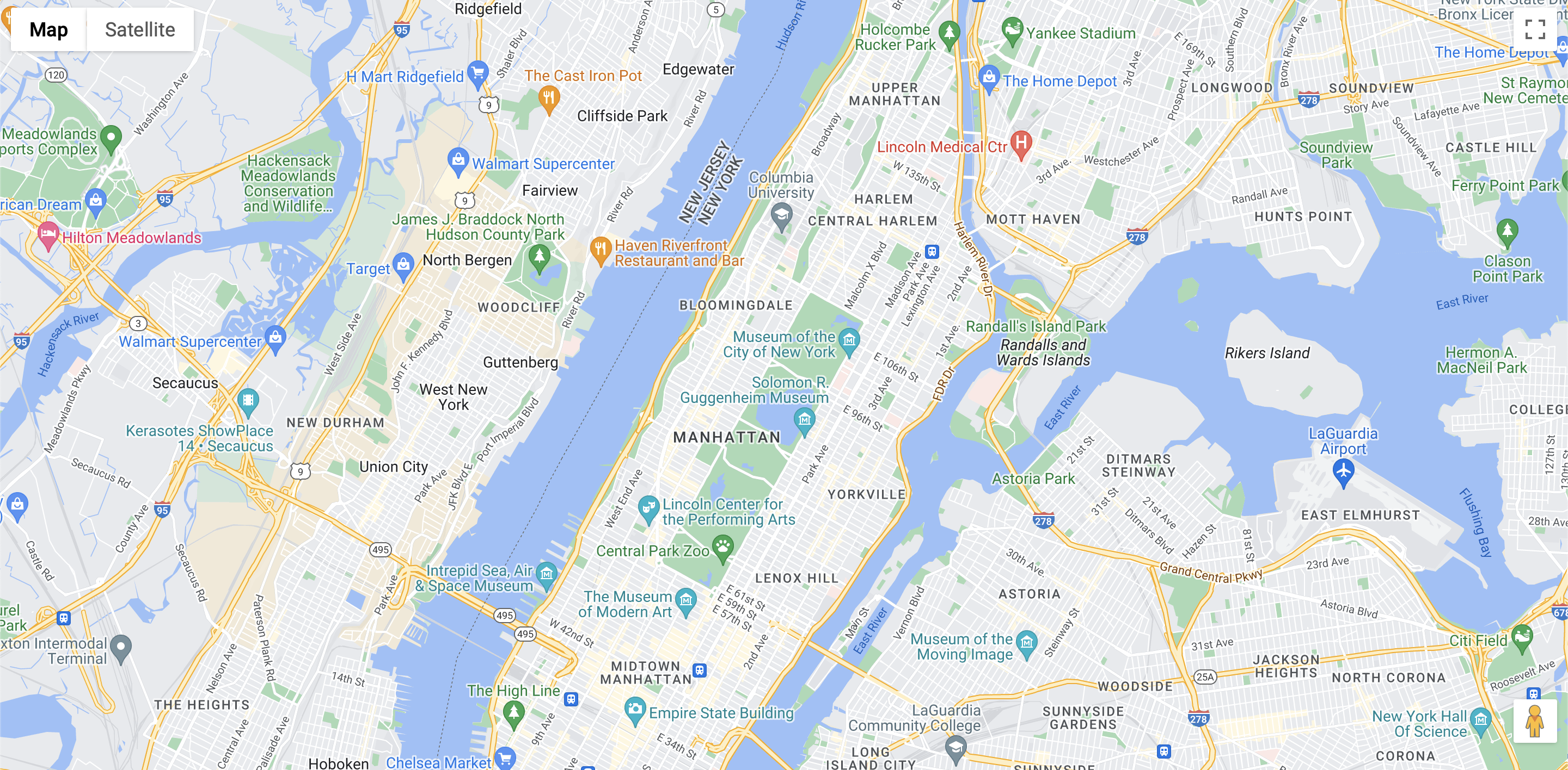 After opening the HTML file in your browser, you can zoom, scroll, change the map to satellite, and mark a spot to see the street-view.
6.2.6 From_Geocode
If you don’t know the exact coordinates you want your map to be centered around you can use the name of the location instead. You do this by attaching the .from_geocode() function to GoogleMapPlotter and inputting a string of the location inside the parenthesis. THIS REQUIRES AN API KEY
Parameters:
- location
str– Location or address of interest, as a human-readable string.
Optional Parameters:
- zoom
int– Zoom level, where 0 is fully zoomed out. Defaults to 13.
# Creating a map centered around the UConn campus
gmap = gmplot.GoogleMapPlotter.from_geocode('UConn, Storrs', 16, apikey=apikey)
gmap.draw('map3.html')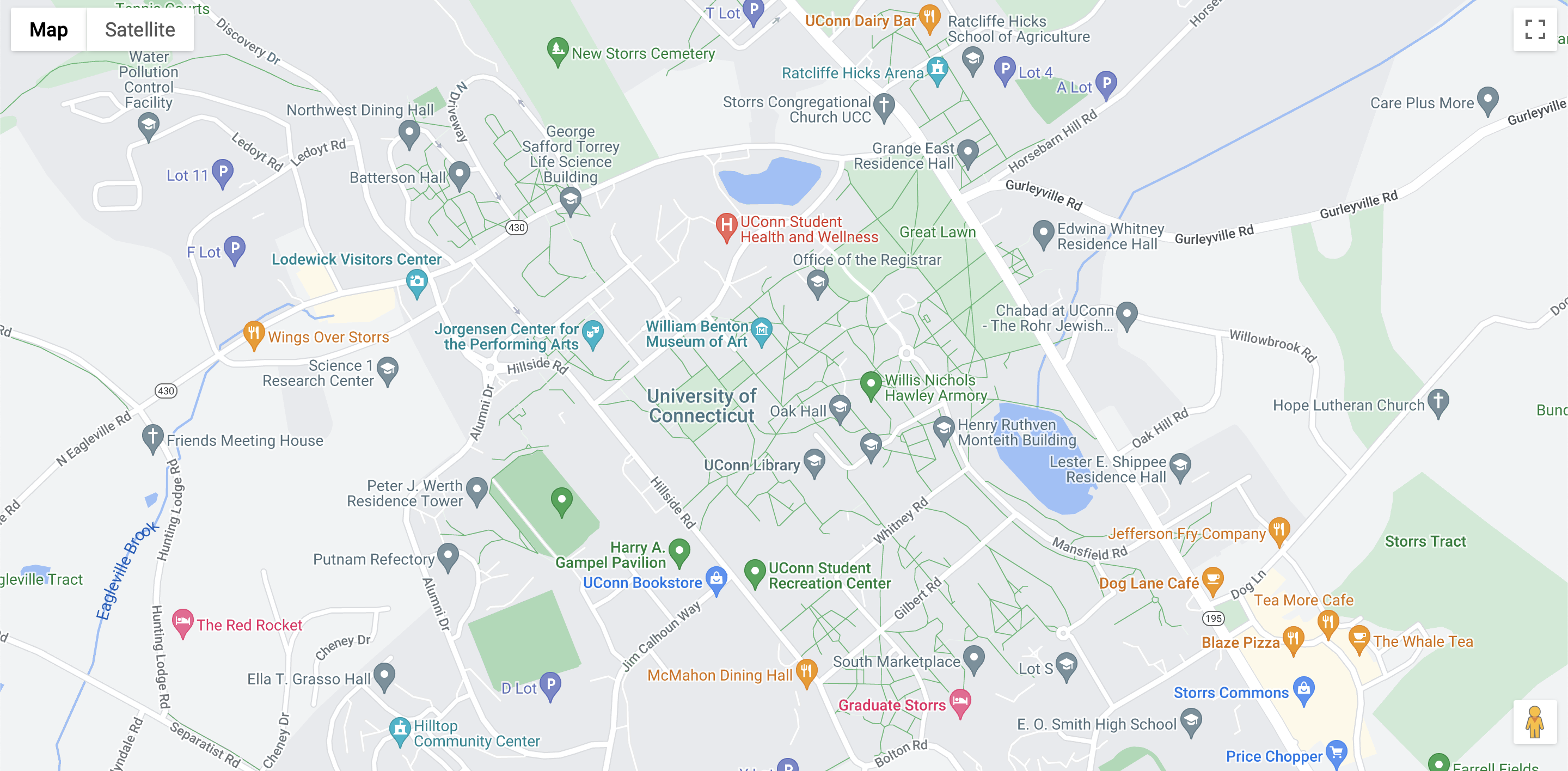
6.2.7 Geocode
If you want to know the latitude and longitude coordinates of a certain location you can use the .geocode() function attached to GoogleMapPlotter. Input a string of said location inside the parenthesis. THIS REQUIRES AN API KEY
# Printing the coordinates of some locations at UConn
uconn = gmplot.GoogleMapPlotter.geocode('UConn, Storrs', apikey=apikey)
garrigus = gmplot.GoogleMapPlotter.geocode('Garrigus Suites, Storrs', apikey=apikey)
gentry = gmplot.GoogleMapPlotter.geocode('Gentry Building, Storrs', apikey=apikey)
print(uconn)
print(garrigus)
print(gentry)(41.8084314, -72.24952309999999)
(41.80522879999999, -72.25755840000001)
(41.8084314, -72.24952309999999)6.2.8 Text on the Map
You can display text labels on your maps using .text()
Parameters:
- lat
float– Latitude of the text label. - lng
float– Longitude of the text label. - text
str– Text to display.
Optional Parameters
- color/c
str– Text color. Can be hex (‘#00FFFF’), named (‘cyan’), or matplotlib-like (‘c’). Defaults to black.
# Map centered around UConn with text labels for Garrigus Suites and the Gentry Building
# Using the coordinates found above
gmap = gmplot.GoogleMapPlotter(uconn[0], uconn[1], 17, apikey=apikey, map_type='hybrid')
# Text labels:
gmap.text(garrigus[0], garrigus[1], 'Garrigus Suites', color='red')
gmap.text(gentry[0], gentry[1], 'Gentry Building', color='orange')
gmap.draw('map4.html')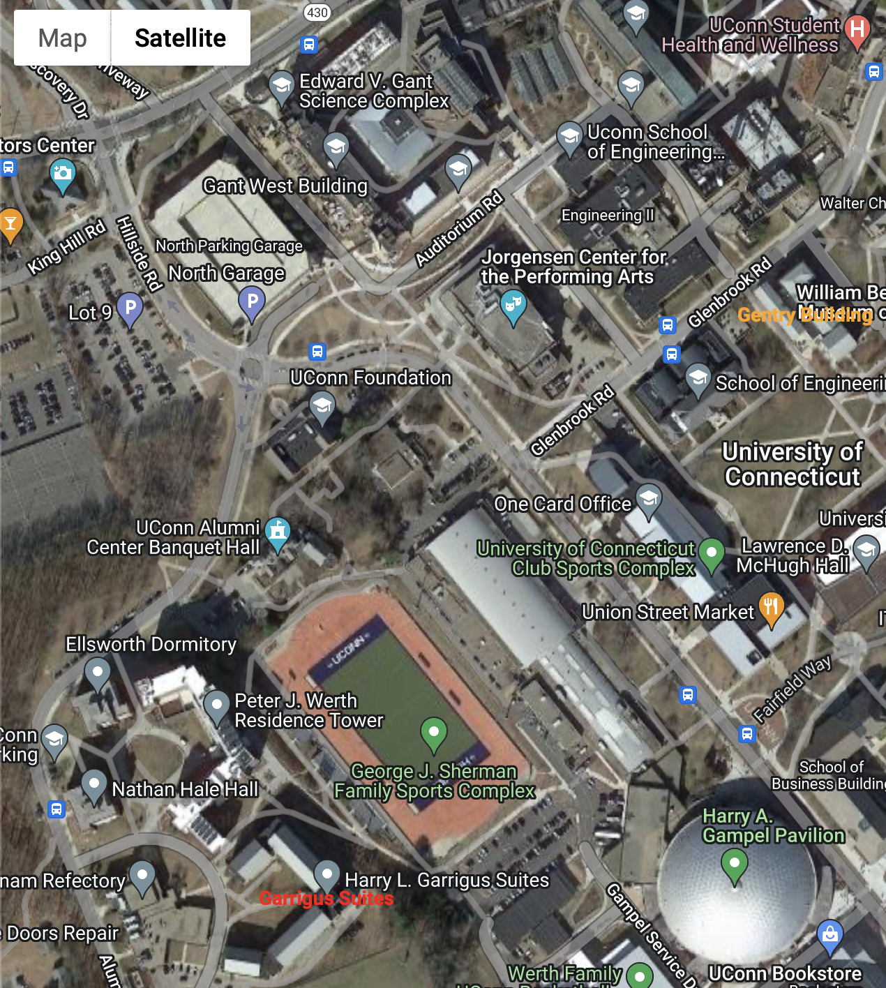
6.2.9 Directions
You can display directions from one location to another on a map using .directions() REQUIRES API KEY
Parameters:
- origin
(float, float)– Origin, in latitude/longitude. - destination
(float, float)– Destination, in latitude/longitude.
Optional Parameters:
- travel_mode
str– Travel mode. Defaults to ‘DRIVING’. - waypoints
[(float, float)]– Waypoints to pass through.
# Walking directions from Garrigus Suites to the Gentry Building
gmap = gmplot.GoogleMapPlotter(uconn[0], uconn[1], 17, apikey=apikey, map_type='hybrid')
# Origin: Garrigus Suites, Destination: Gentry Buldiing
gmap.directions((garrigus[0], garrigus[1]),
(gentry[0], gentry[1]),
travel_mode='WALKING') # walking not driving
gmap.draw('map5.html')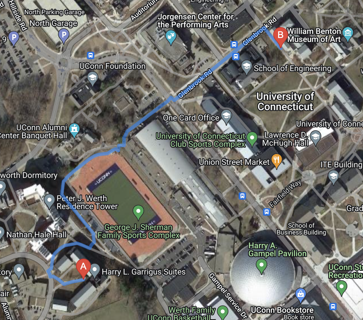
6.2.10 Markers
You can also display markers on the map using .marker(). These markers can contain HTML content in a pop up window.
Parameters:
- lat
float– Latitude of the marker. - lng
float– Longitude of the marker.
Optional Parameters:
- color/c
str– Marker color. Can be hex (‘#00FFFF’), named (‘cyan’), or matplotlib-like (‘c’). Defaults to red. - title
str– Hover-over title of the marker. - precision
int– Number of digits after the decimal to round to for lat/lng values. Defaults to 6. - label
str– Label displayed on the marker. - info_window
str– HTML content to be displayed in a pop-up info window. - draggable
bool– Whether or not the marker is draggable.
gmap = gmplot.GoogleMapPlotter(uconn[0], uconn[1], 17, apikey=apikey)
gmap.marker(garrigus[0], garrigus[1], label='S', info_window=
"<a href='https://reslife.uconn.edu/housing-options/suites/garrigus-suites/'>Garrigus Suites</a")
# Adding Website link to Garrigus Suites on its marker
gmap.marker(gentry[0], gentry[1], color='green', title='Gentry Building') # Marker labeled Gentry Building
gmap.enable_marker_dropping('orange', draggable=True) # Allows you to drop markers on the map by clicking
gmap.draw('map6.html')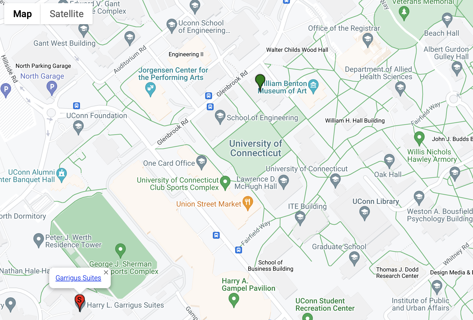
6.2.11 Scatter
You can plot a collection of geographical points on a map using .scatter().
Parameters:
- lats
[float]– Latitudes. - lngs
[float]– Longitudes.
Optional Parameters:
- color/c/edge_color/ec
str– Color of each point. Can be hex (‘#00FFFF’), named (‘cyan’), or matplotlib-like (‘c’). Defaults to black. - size/s
int– Size of each point, in meters (symbols only). Defaults to 40. - marker
bool– True to plot points as markers, False to plot them as symbols. Defaults to True. - symbol
str– Shape of each point, as ‘o’, ‘x’, or ‘+’ (symbols only). Defaults to ‘o’. - title
str– Hover-over title of each point (markers only). - label
str– Label displayed on each point (markers only). - precision
int– Number of digits after the decimal to round to for lat/lng values. Defaults to 6. - alpha/face_alpha/fa
float– Opacity of each point’s face, ranging from 0 to 1 (symbols only). Defaults to 0.3. - alpha/edge_alpha/ea
float– Opacity of each point’s edge, ranging from 0 to 1 (symbols only). Defaults to 1.0. - edge_width/ew
int– Width of each point’s edge, in pixels (symbols only). Defaults to 1.
To illustrate this I will use the cleaned NYC Crash Data, and color each point corresponding to its borough:
# Importing in the cleaned NYC crash data
import pandas as pd
crash = pd.read_csv('data/nyc_crashes_202301_cleaned.csv')# Group the dataframe by the "BOROUGH" column
borough_groups = crash.groupby('BOROUGH')
# Creating a map centered around NYC with the location points scattered
gmap = gmplot.GoogleMapPlotter.from_geocode('New York City', 10, apikey=apikey)
# Loop through each group and plot the points with a different color for each borough
colors = ['red', 'blue', 'green', 'brown', 'purple'] # define a list of colors for each borough
for i, (borough, group) in enumerate(borough_groups):
gmap.scatter(group['LATITUDE'], group['LONGITUDE'], marker=False, size=75, color=colors[i])
# Draw the map
gmap.draw('map7.html')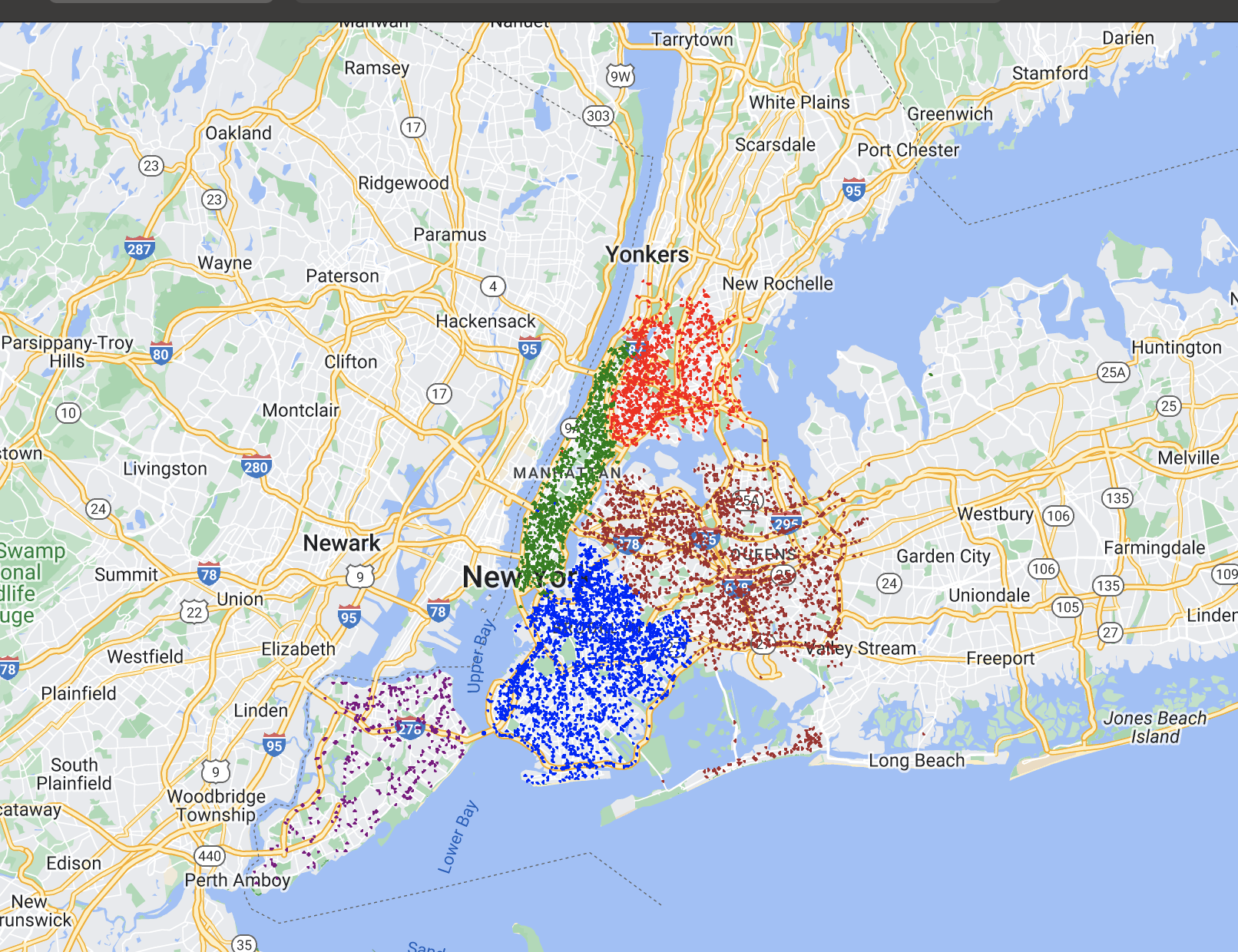
6.2.12 Heatmap and Polygon
You can plot a heatmap of geographical coordinates using .heatmap().
Parameters:
- lats
[float]– Latitudes. - lngs
[float]– Longitudes.
Optional Parameters:
- radius
int– Radius of influence for each data point, in pixels. Defaults to 10. - gradient
[(int, int, int, float)]– Color gradient of the heatmap, as a list of RGBA colors. The color order defines the gradient moving towards the center of a point. - opacity
float– Opacity of the heatmap, ranging from 0 to 1. Defaults to 0.6. - max_intensity
int– Maximum intensity of the heatmap. Defaults to 1. - dissipating
bool– True to dissipate the heatmap on zooming, False to disable dissipation. - precision
int– Number of digits after the decimal to round to for lat/lng values. Defaults to 6. - weights
[float]– List of weights corresponding to each data point. Each point has a weight of 1 by default. Specifying a weight of N is equivalent to plotting the same point N times.
You can also plot a polygon that you can color on a map using .polygon(), using latitude and logitude values of the points of the polygon shape.
Example using same data points as the scatter map above except changing to heatmap. Also plotting a polygon of Central Park:
# You need to drop all na's for heatmap to work
crash_c = crash.dropna(subset=['LATITUDE', 'LONGITUDE'])
# Creating map centered around Manhattan
gmap = gmplot.GoogleMapPlotter.from_geocode("Manhattan, NY", apikey=apikey)
# Coordinates of boundaries of Central Park
centralp = zip(*[
(40.796961, -73.949441),
(40.764684, -73.972968),
(40.767997, -73.981977),
(40.800585, -73.958036)
])
# Heatmap using Crash data coordinates
gmap.heatmap(crash_c['LATITUDE'], crash_c['LONGITUDE'], radius=15, opacity=0.6)
# Blue polygon (rectangle) of Central Park
gmap.polygon(*centralp, face_color='pink', edge_color='cornflowerblue', edge_width=5)
gmap.draw('map8.html')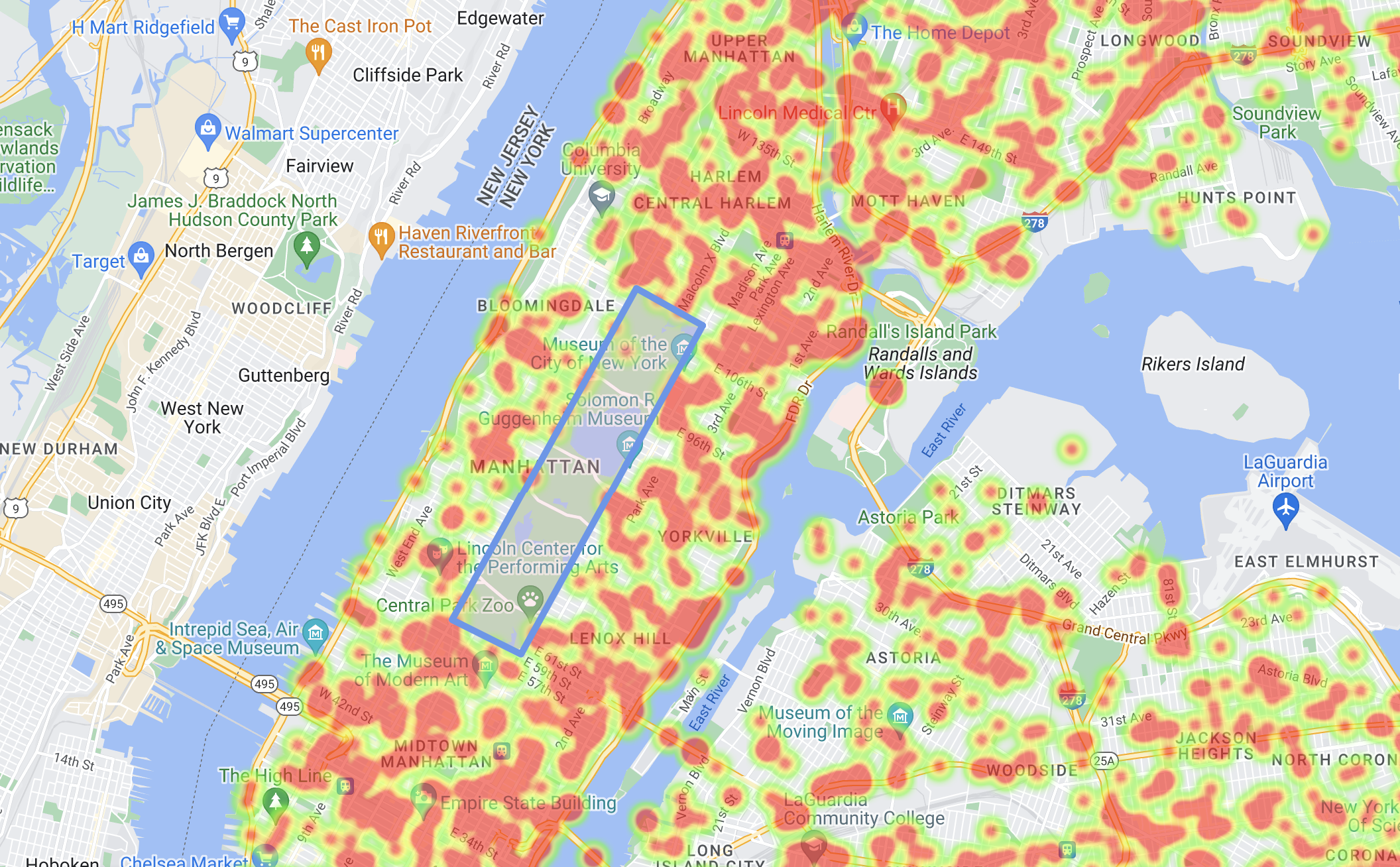
6.2.13 References
Github of gmplot:
Another tutorial website: