Supervised learning uses labeled datasets to train algorithms that to classify data or predict outcomes accurately. As input data is fed into the model, it adjusts its weights until the model has been fitted appropriately, which occurs as part of the cross validation process.
In contrast, unsupervised learning uses unlabeled data to discover patterns that help solve for clustering or association problems. This is particularly useful when subject matter experts are unsure of common properties within a data set.
10.2 Classification vs Regression
Classificaiton: outcome variable is categorical
Regression: outcome variable is continuous
Both problems can have many covariates (predictors/features)
Four rates from the confusion matrix with actual (row) margins:
TPR: TP / (TP + FN). Also known as sensitivity.
FNR: TN / (TP + FN). Also known as miss rate.
FPR: FP / (FP + TN). Also known as false alarm, fall-out.
TNR: TN / (FP + TN). Also known as specificity.
Note that TPR and FPR do not add up to one. Neither do FNR and FPR.
Four rates from the confusion matrix with predicted (column) margins:
PPV: TP / (TP + FP). Also known as precision.
FDR: FP / (TP + FP).
FOR: FN / (FN + TN).
NPV: TN / (FN + TN).
10.2.2.2 Measure of classification performance
Measures for a given confusion matrix:
Accuracy: (TP + TN) / (P + N). The proportion of all corrected predictions. Not good for highly imbalanced data.
Recall (sensitivity/TPR): TP / (TP + FN). Intuitively, the ability of the classifier to find all the positive samples.
Precision: TP / (TP + FP). Intuitively, the ability of the classifier not to label as positive a sample that is negative.
F-beta score: Harmonic mean of precision and recall with \(\beta\) chosen such that recall is considered \(\beta\) times as important as precision, \[
(1 + \beta^2) \frac{\text{precision} \cdot \text{recall}}
{\beta^2 \text{precision} + \text{recall}}
\] See stackexchange post for the motivation of \(\beta^2\).
When classification is obtained by dichotomizing a continuous score, the receiver operating characteristic (ROC) curve gives a graphical summary of the FPR and TPR for all thresholds. The ROC curve plots the TPR against the FPR at all thresholds.
Increasing from \((0, 0)\) to \((1, 1)\).
Best classification passes \((0, 1)\).
Classification by random guess gives the 45-degree line.
Area between the ROC and the 45-degree line is the Gini coefficient, a measure of inequality.
Area under the curve (AUC) of ROC thus provides an important metric of classification results.
10.2.3 Cross-validation
Goal: strike a bias-variance tradeoff.
K-fold: hold out each fold as testing data.
Scores: minimized to train a model
Cross-validation is an important measure to prevent over-fitting. Good in-sample performance does not necessarily mean good out-sample performance. A general work flow in model selection with cross-validation is as follows.
Split the data into training and testing
For each candidate model \(m\) (with possibly multiple tuning parameters)
Fit the model to the training data
Obtain the performance measure \(f(m)\) on the testing data (e.g., CV score, MSE, loss, etc.)
Choose the model \(m^* = \arg\max_m f(m)\).
10.3 Support Vector Machines (by Yang Kang Chua)
10.3.1 Introduction
Support Vector Machine (SVM) is a type of suppervised learning models that can be used to analyze classification and regression. In this section will develop the intuition behind support vector machines and provide some examples.
10.3.2 Package that need to install
Before we begin ensure that these this package are installed in your python
pip install scikit-learn
Scikit-learn is a python package that provides efficient versions of a large number of common algorithms It constist of all type of machine learning model which is wildly known such as:
Linear Regression
Logistic Regression
Decision Trees
Gaussian Process
Furthermore, it also provide function that can be used anytime and use it on the provided machine learning algorithm. There are two type of functions:
Avalable dataset functions such as Iris dataset load_iris
Randomly generated datasets function such as make_moon , make_circle etc.
10.3.3 Support Vector Classifier
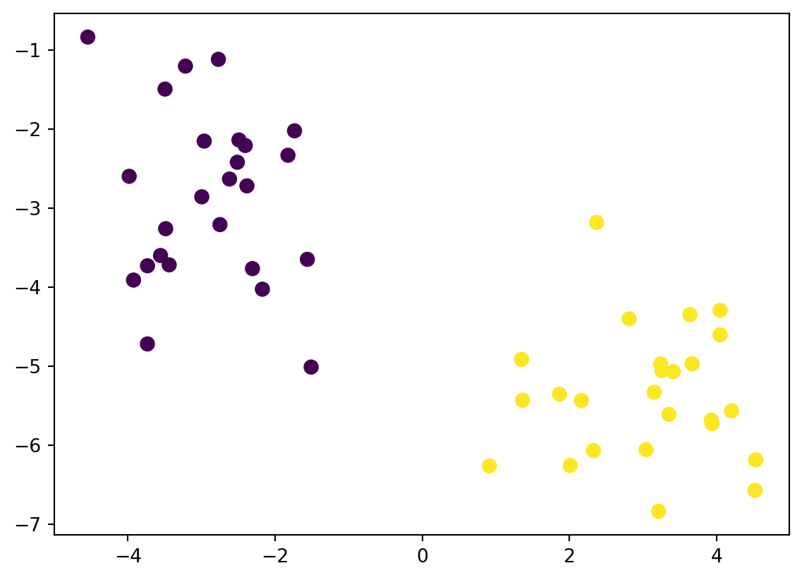
Before we get into SVM , let us take a look at this simple classification problem. Consider a distinguishable datasets
%matplotlib inlineimport numpy as npimport matplotlib.pyplot as pltseed =220from sklearn.datasets import make_blobsX, y = make_blobs(n_samples=50, centers=2, random_state= seed, cluster_std=1)plt.scatter(X[:, 0], X[:, 1], c=y, s=50);
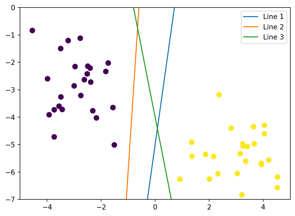
One of the solution we can do is to draw lines as a way to seperate these two classes.
How do we find the best line that divide them both? In other word we need to find the optimal line or best decision boundary.
Lets import Support Vector Machine module for now to help us find the best line to classify the data set.
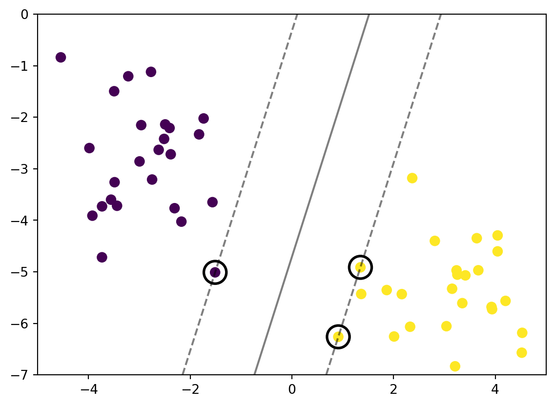
from sklearn.svm import SVC # "Support vector classifier"model = SVC(kernel='linear', C=1E10)# For now lets not think about the purpose of Cmodel.fit(X, y)ax = plt.gca()ax.set_xlim(-5, 5)ax.set_ylim(-7, 0)xlim = ax.get_xlim()ylim = ax.get_ylim()# Create a mesh gridx_grid = np.linspace(xlim[0], xlim[1], 30)y_grid = np.linspace(ylim[0], ylim[1], 30)Y_mesh, X_mesh = np.meshgrid(y_grid,x_grid)xy = np.vstack([X_mesh.ravel(),Y_mesh.ravel()]).TP = model.decision_function(xy).reshape(X_mesh.shape)ax.contour(X_mesh, Y_mesh, P, colors='k', levels=[-1, 0 ,1], alpha=0.5, linestyles= ['--','-','--']);ax.scatter(X[:, 0], X[:, 1], c=y, s=50);ax.scatter(model.support_vectors_[:, 0], model.support_vectors_[:, 1], s=300, linewidth=2, facecolor ='none', edgecolor ='black');
There is a name for this line. Is called margin, it is the shortest distance between the selected observation and the line. In this case we are using the largest margin to seperate the observation. We called it Maximal Margin Classifier.
The selected observation (circled points) are called Support Vectors. For simple explaination, it is the points that used to create the margin.
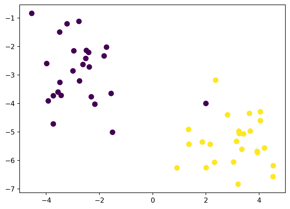
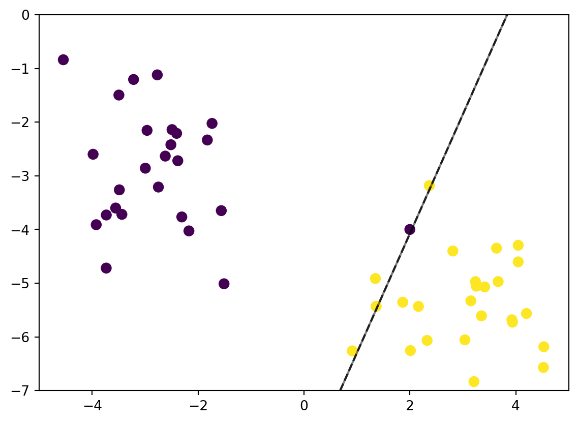
What if we have a weird observation as shown below? What happend if we try to use Maximal Margin Classifier? Lets add a point on an interesting location.
# Addiing a point near yellow side and name it bluefrom sklearn.datasets import make_blobsX, y = make_blobs(n_samples=50, centers=2, random_state=220, cluster_std=1)X_new = [2, -4]X = np.vstack([X,X_new])y_new = np.array([1]).reshape(1)y = np.append(y, [0], axis=0)ax = plt.subplot()ax.scatter(X[:, 0], X[:, 1], c=y, s=51);
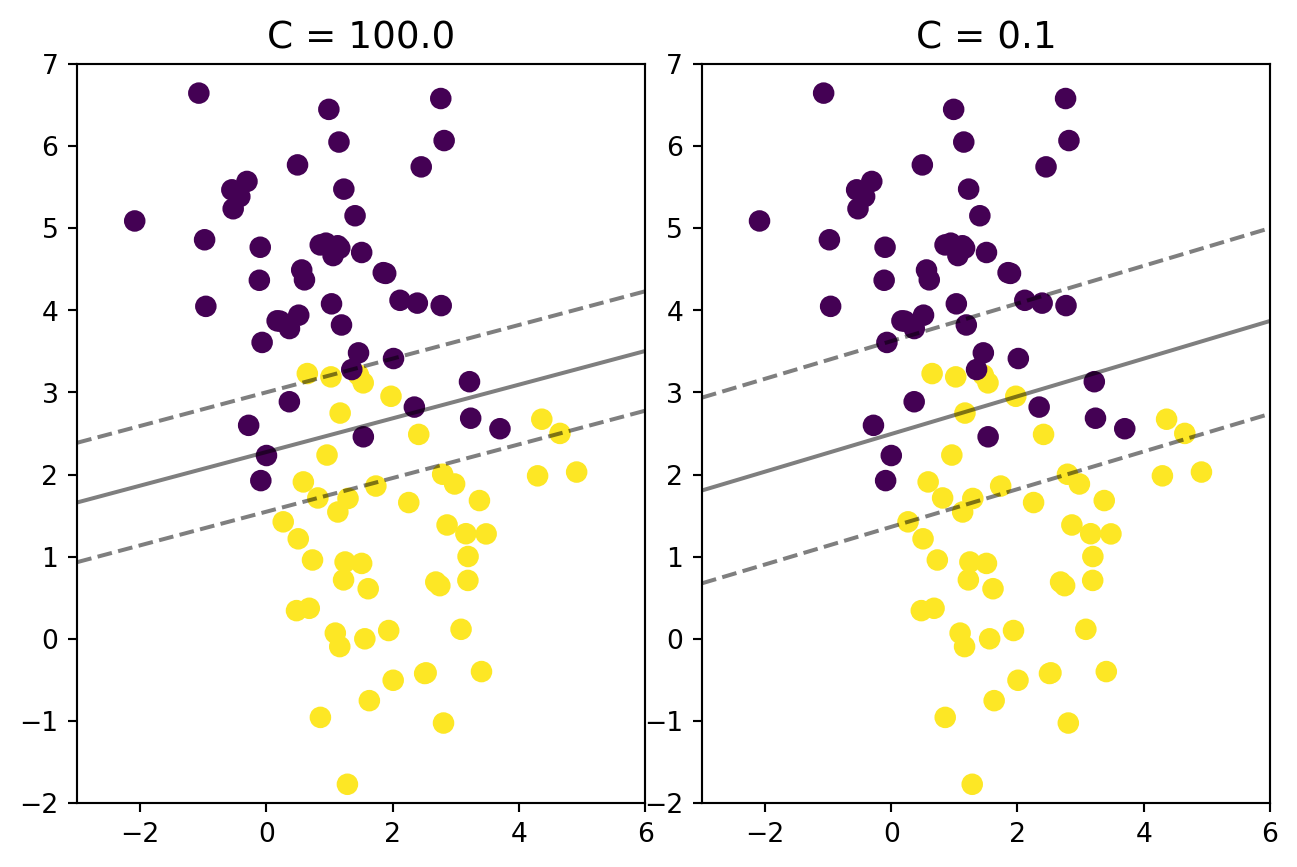
As you can see Maximal Margin Classifier might not be a useful in this case. We must make the margin that is not sensitve to outliers and allow a few misclassifications. So we need to implement Soft Margin to get a better prediction. This is where parameter C comes in.
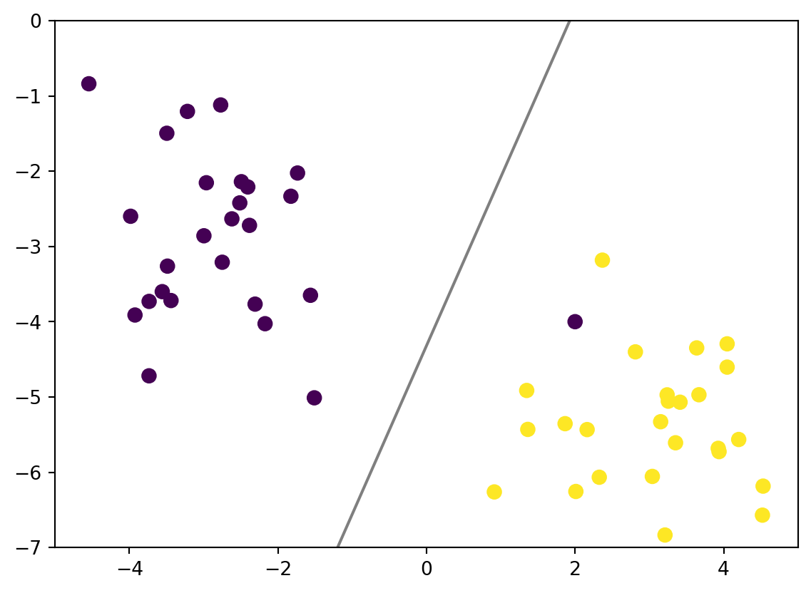
# New fit with modifiying the Cmodel = SVC(kernel='linear', C=0.1)model.fit(X, y)ax = plt.gca()ax.set_xlim(-5, 5)ax.set_ylim(-7, 0)xlim = ax.get_xlim()ylim = ax.get_ylim()# Create a mesh gridx_grid = np.linspace(xlim[0], xlim[1], 30)y_grid = np.linspace(ylim[0], ylim[1], 30)Y_mesh, X_mesh = np.meshgrid(y_grid,x_grid)xy = np.vstack([X_mesh.ravel(),Y_mesh.ravel()]).TP = model.decision_function(xy).reshape(X_mesh.shape)ax.contour(X_mesh, Y_mesh, P, colors='k', levels=0, alpha=0.5, linestyles='-');ax.scatter(X[:, 0], X[:, 1], c=y, s=50);
Increasing the parameter C will greatly influence the classification line location
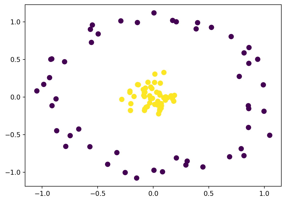
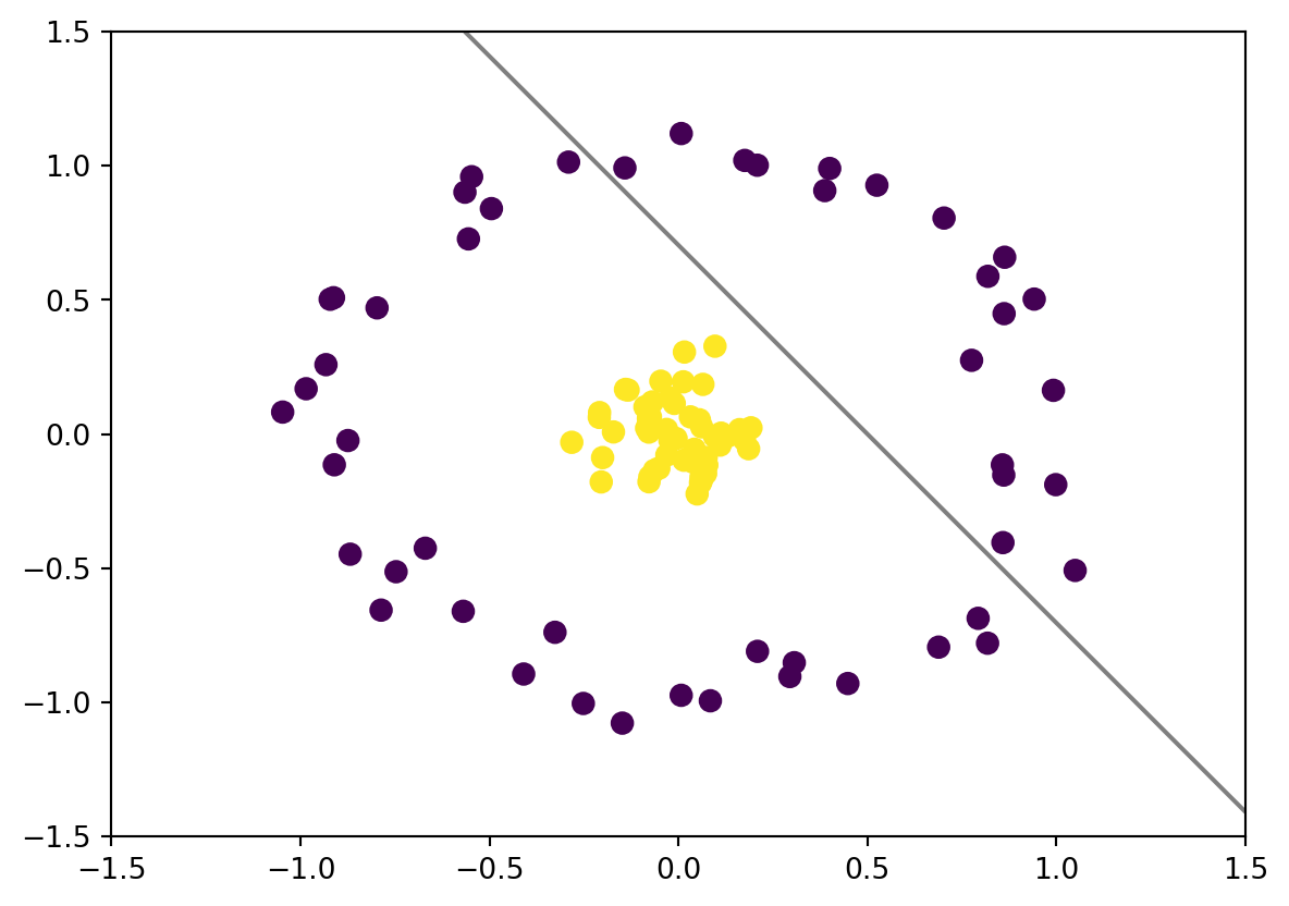
This is not a good classifier. We need a way to make it better. Instead of just using the available data, let us try to convert a data to a better dimension space.
r = np.exp(-(X **2).sum(1))
In this case we will implement a kernel that will translate our data to a new diemension. This is one of the way to fit a nonlinear relationship with a linear classifier.
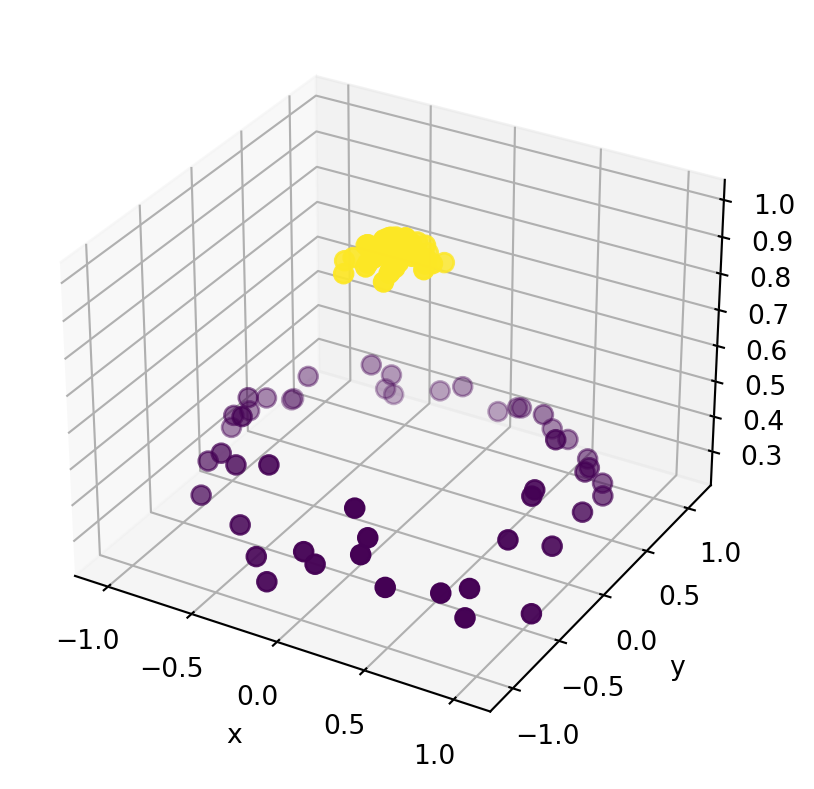
As for summary, Support Vector Machine follow these steps:
Start with a data in low dimension.
Use kernel to move the data to a higher dimension.
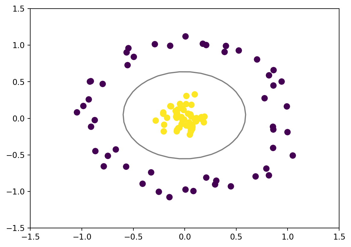
Find a Support Vector Classifier that seperate the data into two groups.
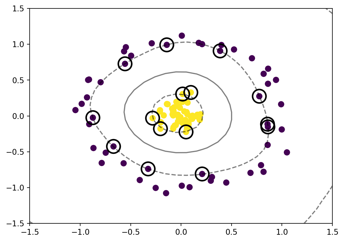
10.3.3.2 Kernel
Let talk more about the kernel. There are mutiple type of kernel. We will go through a few of them. Generaly, they call as a kernel trick or kernel method or kernel function. For simple explanation, these kernel can be view as a method on how we transform the data points into. It may need to transform to a higher dimension it may not.
Linear Kernel The linear kernel is a kernel that uses the dot product of the input vectors to measure their similarity: \[k(x,x')= (x\cdot x')\]
Polynomial Kernel
For homogeneous case: \[k(x,x')= (x\cdot x')^d\] where if \(d = 1\) it wil be act as linear kernel.
For inhomogeneous case: \[k(x,x')= (x\cdot x' + r )^d\] where r is a coefficient.
Radial Basis Function Kernel (or rbf) is a well know kernel that can transform the data to a infinite dimension space.
\(\gamma >0\). Sometimes parametrized using \(\gamma = \frac{1}{2\sigma^2}\)
10.3.3.3 Regression Problem
We will talk a little on Regression Problem and how it works on Support Vector Machine.
Lets consider a data output as shown below.
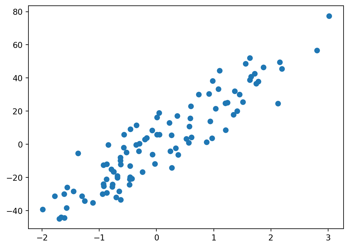
from sklearn.datasets import make_regressionimport matplotlib.pyplot as pltX, y = make_regression(n_samples=100, n_features=1, noise=10, random_state =2220)plt.scatter(X, y, marker='o')plt.show()
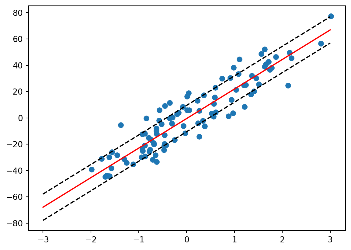
So how Support Vector Machine works for regression problem? Instead of giving some math formulas. Let do a fit and show the output of the graph.
As you can see for regression problem Support Vector Machine for Regression or SVR create a two black lines as the decision boundary and the red line as the hyperplane. Our objective is to ensure points are within the boundary. The best fit line is the hyperplane that has a maximum number of points.
You can control the model by adjust the C value and epsilon value. C value change the slope of the line, lower the value will reduce the slope of the fit line. epsilon change the distance of the decision boundary, lower the epsilon reduce the distance of the dicision boundary.
10.3.3.4 Example: Classification
Let take a look at our NYC database. We would like to create a machine learning model with SVM.
import pandas as pdjan23 = pd.read_csv("data/nyc_crashes_202301_cleaned.csv")jan23.head()
CRASH DATE
CRASH TIME
BOROUGH
ZIP CODE
LATITUDE
LONGITUDE
LOCATION
ON STREET NAME
CROSS STREET NAME
OFF STREET NAME
...
Unnamed: 30
Unnamed: 31
Unnamed: 32
Unnamed: 33
Unnamed: 34
Unnamed: 35
Unnamed: 36
Unnamed: 37
Unnamed: 38
Unnamed: 39
0
1/1/23
14:38
BROOKLYN
11211.0
40.719094
-73.946108
(40.7190938,-73.9461082)
BROOKLYN QUEENS EXPRESSWAY RAMP
NaN
NaN
...
NaN
NaN
NaN
NaN
NaN
NaN
NaN
NaN
NaN
NaN
1
1/1/23
8:04
QUEENS
11430.0
40.659508
-73.773687
(40.6595077,-73.7736867)
NASSAU EXPRESSWAY
NaN
NaN
...
NaN
NaN
NaN
NaN
NaN
NaN
NaN
NaN
NaN
NaN
2
1/1/23
18:05
MANHATTAN
10011.0
40.742454
-74.008686
(40.7424543,-74.008686)
10 AVENUE
11 AVENUE
NaN
...
NaN
NaN
NaN
NaN
NaN
NaN
NaN
NaN
NaN
NaN
3
1/1/23
23:45
QUEENS
11103.0
40.769737
-73.912440
(40.769737, -73.91244)
ASTORIA BOULEVARD
37 STREET
NaN
...
NaN
NaN
NaN
NaN
NaN
NaN
NaN
NaN
NaN
NaN
4
1/1/23
4:50
BRONX
10462.0
40.830555
-73.850720
(40.830555, -73.85072)
CASTLE HILL AVENUE
EAST 177 STREET
NaN
...
NaN
NaN
NaN
NaN
NaN
NaN
NaN
NaN
NaN
NaN
5 rows × 40 columns
Let us merge with uszipcode database to increase the number of input value to predict injury.
#Calculate the sumjan23['sum'] = jan23['NUMBER OF PERSONS INJURED'] + jan23['NUMBER OF PEDESTRIANS INJURED']+ jan23['NUMBER OF CYCLIST INJURED'] + jan23['NUMBER OF MOTORIST INJURED']for index in jan23.index:if jan23['sum'][index] >0: jan23.loc[index,['injured']] =1else: jan23.loc[index,['injured']] =0from uszipcode import SearchEnginesearch = SearchEngine()resultlist = []for index in jan23.index: checkZip = jan23['ZIP CODE'][index]if np.isnan(checkZip) ==False: zipcode =int(checkZip) result = search.by_zipcode(zipcode) resultlist.append(result.to_dict())else: resultlist.append({})Zipcode_data = pd.DataFrame.from_records(resultlist)merge = pd.concat([jan23, Zipcode_data], axis=1)# Drop the repeated zipcodemerge = merge.drop(['zipcode','lat','lng'],axis =1)merge = merge[merge['population'].notnull()]Focus_data = merge[['radius_in_miles', 'population', 'population_density','land_area_in_sqmi', 'water_area_in_sqmi', 'housing_units','occupied_housing_units','median_home_value','median_household_income','injured']]
These are the focus data that we will apply SVM to.
Focus_data.head()
radius_in_miles
population
population_density
land_area_in_sqmi
water_area_in_sqmi
housing_units
occupied_housing_units
median_home_value
median_household_income
injured
0
2.000000
90117.0
39209.0
2.30
0.07
37180.0
33489.0
655500.0
46848.0
1.0
2
0.909091
50984.0
77436.0
0.66
0.00
33252.0
30294.0
914500.0
104238.0
0.0
3
0.852273
38780.0
54537.0
0.71
0.00
18518.0
16890.0
648900.0
55129.0
1.0
4
1.000000
75784.0
51207.0
1.48
0.00
31331.0
29855.0
271300.0
45864.0
0.0
5
2.000000
80018.0
36934.0
2.17
0.05
34885.0
30601.0
524100.0
51725.0
0.0
To reduce the complexity, we will get 1000 sample from the dataset and import train_test_split to split up our data to measure the performance.
random_sample = Focus_data.sample(n=1000, random_state=220)#Create X inputX = random_sample[['radius_in_miles', 'population', 'population_density','land_area_in_sqmi', 'water_area_in_sqmi', 'housing_units','occupied_housing_units','median_home_value','median_household_income']].values#Create Y for outputy = random_sample['injured'].valuesfrom sklearn.model_selection import train_test_split X_train, X_test, y_train, y_test = train_test_split(X, y, test_size =0.20)
Apply SVM to our dataset and make a prediction on X_test
from sklearn.svm import SVC clf = SVC(kernel='rbf').fit(X_train, y_train)#Make prediction using X_testy_pred = clf.predict(X_test)
Check our accuracy of our model by importing accuracy_score from sklearn.metrics
from sklearn.metrics import accuracy_scoreaccuracy = accuracy_score(y_test, y_pred)accuracy
0.655
10.3.4 Conclusion
Support Vector Machines is one of the powerful tool mainly for classifications.
Their dependence on relatively few support vectors means that they are very compact models, and take up very little memory.
Once the model is trained, the prediction phase is very fast.
Because they are affected only by points near the margin, they work well with high-dimensional data—even data with more dimensions than samples, which is a challenging regime for other algorithms.
Their integration with kernel methods makes them very versatile, able to adapt to many types of data.
However, SVMs have several disadvantages as well:
The scaling with the number of samples \(N\) is \(O[N^3]\) at worst, or \(O[N^2]\) for efficient implementations. For large numbers of training samples, this computational cost can be prohibitive.
The results are strongly dependent on a suitable choice for the softening parameter \(C\).This must be carefully chosen via cross-validation, which can be expensive as datasets grow in size.
The results do not have a direct probabilistic interpretation. This can be estimated via an internal cross-validation (see the probability parameter of SVC), but this extra estimation is costly.
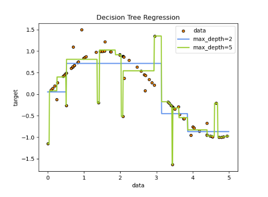
Decision Trees (DTs) are a non-parametric supervised learning method used for classification and regression. The goal is to create a model that predicts the value of a target variable by learning simple decision rules inferred from the data features. A tree can be seen as a piecewise constant approximation.
For instance, in the example below, decision trees learn from data to approximate a sine curve with a set of if-then-else decision rules. The deeper the tree, the more complex the decision rules and the fitter the model.
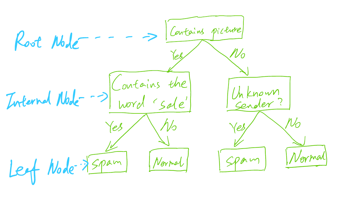
Both root and internal nodes have child nodes that branch out from them based on the value of a feature. For instance, the root node splits the unknown_sender feature space, and the threshold is 0.5. Its left subtree represents all the data with unknown_sender <= 0.5, whereas its right subtree represents all the subset of data with unknown_sender > 0.5. Each leaf node has an predicted value which will be used as the output from the decision tree. For example, the leftmost leaf node (left child of the root node) will lead to output is_spam = 0 (i.e. “normal”).
We can use this model to make some prediction.
new_email_feat = [[0, 1, 0], # Known sender, contains sales word, no scam word [1, 1, 0]] # Unknown sender, contains sales word, no scam wordclf.predict(new_email_feat) # expected result: 0 (normal), 1 (spam)
array([0, 1])
Given an input, the predicted outcome is obtained by traversing the decision tree. The traversal starts from the root node, and chooses left or right subtree based on the node’s splitting rule recursively, until it reaches a leaf node.
For the example input [1, 1, 0], its unknown_sender feature is 1, so we follow the right subtree based on the root node’s splitting rule. The next node splits on the scam_words feature, and since its value is 0, we follow the left subtree. The next node uses the sales_words feature, and its value is 1, so we should go down to the right subtree, where we reach a leaf node. Thus the predicted outcome is the value 1 (class “spam”).
10.4.2 Tree algorithms
As many other supervised learning approaches, the decision trees are constructed in a way that minimizes a chosen cost function. It is computationally infeasible to find the optimal decision tree that minimizes the cost function. Thus, a greedy approach known as recursive binary splitting is often used.
Package scikit-learn uses an optimized version of the CART algorithm; however, the scikit-learn implementation does not support categorical variables for now. Minimal cost-complexity pruning is an algorithm used to prune a tree to avoid over-fitting.
10.4.2.1 Cost function
Gini and entropy are classification criteria. Mean Squared Error (MSE or L2 error), Poisson deviance and Mean Absolute Error (MAE or L1 error) are Regression criteria. Here shows the mathematical formulations to get gini and entropy.
As we see from the above example, in a decision tree, each tree node \(m\) is associated with a subset of the training data set. Assume there are \(n_m\) data points associated with \(m\), and the class values of the data points are in the set \(Q_m\).
Further assume that there are K classes, and let \[
p_{mk}=\frac{1}{n_m}\sum_{y\in Q_m}I(y=k) (k=1,...,K)
\] represent the proportion of class \(k\) observations in node \(m\). Then the cost functions (referred to as classification criteria in sklearn) available in sklearn are: * Gini: \[
H(Q_m)=\sum_{k}p_{mk}(1-p_{mk})
\] * Log loss or entropy: \[
H(Q_m)=-\sum_{k}p_{mk}log(p_{mk})
\]
In sklearn.tree.DecisionTreeClassifierhe, the default criterion is gini. One advantage of using Gini impurity over entropy is that it can be faster to compute, since it involves only a simple sum of squares rather than logarithmic functions. Additionally, Gini impurity tends to be more robust to small changes in the data, while entropy can be sensitive to noise.
10.4.2.2 How to choose what feature and threshold to split on at each node?
The decision tree algorithm iterates over all possible features and thresholds and chooses the one that maximize purity or minimize impurity or maximize information gain.
Let’s use the spam email example to calulate the impurity reduction.
The impurity reduction based on Gini is calculated as the difference between the Gini index of the parent node and the weighted average of the Gini of the child nodes. The split that results in the highest impurity reduction based on Gini is chosen as the best split.
clf_graph
10.4.2.3 When to stop splitting?
There are several stopping criteria that can be used to decide when to stop splitting in a decision tree algorithm. Here are some common ones:
When a node is 100% one class
Maximum depth: Stop splitting when the tree reaches a maximum depth, i.e., when the number of levels in the tree exceeds a predefined threshold.
Minimum number of samples: Stop splitting when the number of samples in a node falls below a certain threshold. This can help avoid overfitting by preventing the tree from making very specific rules for very few samples.
Minimum decrease in impurity: Stop splitting when the impurity measure (e.g., Gini impurity or entropy) does not decrease by a certain threshold after a split. This can help avoid overfitting by preventing the tree from making splits that do not significantly improve the purity of the resulting child nodes.
Maximum number of leaf nodes: Stop splitting when the number of leaf nodes reaches a predefined maximum.
from sklearn import treeimport pandas as pdimport numpy as np
10.4.3.1.3 Step 3: Preparing the Data
NYC = pd.read_csv("data/merged.csv")
# drop rows with missing data in some columnsNYC = NYC.dropna(subset=['BOROUGH', 'hour', 'median_home_value', 'occupied_housing_units'])# Select the featuresnyc_subset = NYC[['BOROUGH', 'hour', 'median_home_value', 'occupied_housing_units']].copy()
# One hot encode categorical featuresnyc_encoded = pd.get_dummies(nyc_subset, columns=['BOROUGH', 'hour'])nyc_encoded
# Fit the model and plot the tree (using default parameters)injury_clf = tree.DecisionTreeClassifier( criterion='gini', splitter='best', max_depth=None, min_samples_split=2, min_samples_leaf=1, min_weight_fraction_leaf=0.0, max_features=None, max_leaf_nodes=None, min_impurity_decrease=0.0, class_weight=None, ccp_alpha=0.0)injury_clf = injury_clf.fit(X_train, y_train)
injury_clf.tree_.node_count
3537
Arguments related to stopping criteria: * max_depth * min_samples_split * min_samples_leaf * min_weight_fraction_leaf * max_features * max_leaf_nodes * min_impurity_decrease
Other important arguments: * criterion: cost function to use * splitter: node splitting strategy * ccp_alpha: pruning parameter
from sklearn.model_selection import GridSearchCV# define the hyperparameter grid for logistic regressionparam_grid = {'criterion': ['gini', 'entropy'],'max_depth': [10, 15, 20],'min_impurity_decrease': [1e-4, 1e-3, 1e-2],'ccp_alpha': [0.0, 1e-5, 1e-4, 1e-3]}# perform cross-validation with GridSearchCVtree_clf = tree.DecisionTreeClassifier()grid_search = GridSearchCV(tree_clf, param_grid, cv=5, scoring='f1')# fit the GridSearchCV object to the training datagrid_search.fit(X_train, y_train)# print the best hyperparameters foundgrid_search.best_params_
In conclusion, decision trees are a widely used supervised learning algorithm for classification and regression tasks. They are easy to understand and interpret. The algorithm works by recursively splitting the dataset based on the attribute that provides the most information gain or the impurity reduction. The tree structure is built from the root node to the leaf nodes, where each node represents a decision based on a feature of the data.
One advantage of decision trees is their interpretability, which allows us to easily understand the decision-making process. They can also model complex problems with multiple outcomes. They are not affected by missing values or outliers.
However, decision trees can be prone to overfitting and may not perform well on complex datasets. They can also be sensitive to small variations in the training data and may require pruning to prevent overfitting. Random forest would be a better choice in this situation. Furthermore, decision trees may not perform well on imbalanced datasets, and their performance can be affected by the selection of splitting criteria.
Overall, decision trees are a useful and versatile tool in machine learning, but it is important to carefully consider their advantages and disadvantages before applying them to a specific problem.
Random forest (RF) is a commonly-used ensemble machine learning algorithm. It is a bagging, also known as bootstrap aggregation, method, which combines the output of multiple decision trees to reach a single result.
Regression: mean
Classification: majority vote
10.5.1 Algorithm
RF baggs on both data (rows) and features (columns).
A random sample of the training data in a training set is selected with replacement (bootstrap)
A random subset of the features is selected as features (which ensures low correlation among the decision trees)
Hyperparameters
node size
number of trees
number of features
Use cross-valudation to select the hyperparameters.
Advantages:
Reduced risk of overfitting since averaging of uncorrelated trees lowers overall variance and prediction error.
Provides flexibility in handeling missing data.
Easy to evaluate feature importance
Mean decrease in impurity (MDI): when a feature is excluded
Mean decrease accuracy: when the values of a feature is randomly permuted
Disadvantages:
Computing intensive
Resource hungery
Interpretation
10.6 Bagging vs. Boosting (by Nathan Nhan)
10.6.1 Introduction
Before we talk about Bagging and Boosting we first must talk about ensemble learning. Ensemble learning is a technique used in machine-learning where we have multiple models (often times called “weak learners”) that are trained to solve the same problem and then combined to obtain better results that they could individually. With this, we can obtain more accurate and more robust models for our data using this technique.
Bagging and boosting are two types of ensemble learning techniques. They decrease the variance of a single estimate as they combine multiple estimates from different models to create a model with higher stability. Additionally, ensemble learning techniques increase the stability of the final model by reducing faactors of error in our models such as unnecessary noise, bias, and variance that we might find hurts the accuracy of our model. Specifically:
Bagging helps decrease the model’s variance and prevent over-fitting.
Boosting helps decrease the model’s bias.
10.6.2 Bagging
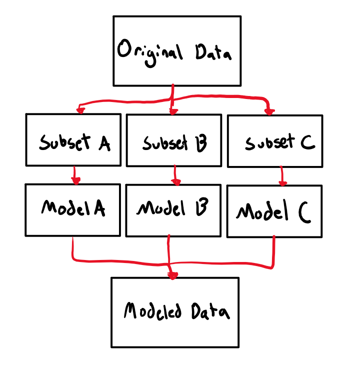
Bagging, which stands for bootrap aggregation, is a ensemble learning algorithm designed to improve the stability and accuracy of algorithms used in statistical classification and regression. In Bagging, multiple homogenous algorithms are trained independently and combined afterward to determine the model’s average. It works like this:
From the original dataset, multiple subsets are created, selecting observations with replacement.
On each of these subsets, a base learner (weak learner) is created for each
Next, all the independent models are run in parallel with one another
The final predictions are determined by combining the predictions from all the models.
Visualization on how the bagging algorithm works
The benefits of using bagging algorithms are that * Bagging algorithms reduce bias and variance errors. * Bagging algorithms can handle overfitting (when a model works with a training dataset but fails with the actual testing dataset). * Bagging can easily be implemented and produce more robust models.
10.6.2.1 Illustration
First we must load the dataset. For this topic I will be generating a madeup dataset shown below. It is recommended to make sure the dataset has no missing values as datasets with missing values leads to inconsistent results and poor model performance.
import pandas as pdimport numpy as npimport randomlength =1000random.seed(0)# Generate a random datasetdata = {'Age': [random.randint(10, 80) for x inrange(length)],'Weight': [random.randint(110, 250) for x inrange(length)],'Height': [random.randint(55, 77) for x inrange(length)],'Average BPM': [random.randint(70, 100) for x inrange(length)],'Amount of Surgeries': [random.randint(0, 3) for x inrange(length)],'Blood Pressure': [random.randint(100, 180) for x inrange(length)], }data['Healthy?'] = np.nandf = pd.DataFrame(data)# Generate a random response variable displaying "1" for healthy and "0" for unhealthyfor index, row in df.iterrows():if row['Blood Pressure'] <110and row['Average BPM'] >80: df.at[index, 'Healthy?'] = random.choice([0, 1, 1, 1, 0, 0, 0])else: df.at[index, 'Healthy?'] = random.choice([1, 1, 1, 1, 0, 1, 1, 1, 1, 1, 1])df
Age
Weight
Height
Average BPM
Amount of Surgeries
Blood Pressure
Healthy?
0
59
125
61
92
1
177
1.0
1
63
198
71
72
0
149
1.0
2
15
218
72
74
0
117
1.0
3
43
144
66
96
3
132
1.0
4
75
165
69
84
3
173
1.0
...
...
...
...
...
...
...
...
995
15
113
73
74
2
147
1.0
996
11
184
63
74
3
102
1.0
997
38
139
73
72
1
110
1.0
998
51
152
68
99
0
159
1.0
999
18
180
56
80
1
162
1.0
1000 rows × 7 columns
Next, we need to specify the x and y variables where the x-variable will hold all the input columns containing numbers and y-variable will contain the output column.
X = df.drop(["Healthy?"], axis="columns")y = df['Healthy?']print(X)
Next we must scale our data. Dataset scaling is transforming the dataset to fit within a specific range. This ensures that no data point is left out during model training. In the example giving we will use the StandardScaler method to scale our dataset.
from sklearn.preprocessing import StandardScalerscaler = StandardScaler()X_scaled = scaler.fit_transform(X)print(X)print(X_scaled)
After scaling the dataset, we can split it. We will split the scaled dataset into two subsets: training and testing. To split the dataset, we will use the train_test_split method. We will be using the default splitting ratio for the train_test_split method which means that 80% of the data will be the training set and 20% the testing set.
from sklearn.model_selection import train_test_splitX_train, X_test, y_train, y_test = train_test_split(X_scaled, y, stratify=y, random_state=0)
Now that we have split our data, we can now perform our classification. The BaggingClassifier classifier will perform all the bagging steps and build an optimized model based on our data. The BaggingClassifier will fit the weak/base learners on the randomly sampled subsets. The listed parameters are as follows:
estimator - this parameter takes the algoithm we want to use, in this example we use the DecisionTreeClassifier for our weak learners.
n_estimators - this parameter takes the amount of weak learners we want to use.
max_samples - this parameter represents The maximum number of data that is sampled from the training set. We use 80% of the training dataset for resampling.
bootstrap - this parameter allows for resampling of the training dataset without replacement when set to True.
oob_score - this parameter is used to compute the model’s accuracy score after training.
random_state - Seed used by the random number generator so we can reproduce out results
from sklearn.ensemble import BaggingClassifierfrom sklearn.tree import DecisionTreeClassifierbag_model = BaggingClassifier(estimator=DecisionTreeClassifier(), # DecisionTreeClassifier() if estimator is not definedn_estimators=100, bootstrap=True,oob_score=True,random_state =0)bag_model.fit(X_train, y_train)AccScore = bag_model.oob_score_print("Accuracy Score for Bagging Classifier: "+str(AccScore))
Accuracy Score for Bagging Classifier: 0.8853333333333333
We can find if overfitting occurs when we get a lower accuracy when using the testing dataset. We can find this by running the following code:
if bag_model.score(X_test, y_test) < AccScore:print('Overfitting has occurred since the testing dataset has a lower accuracy than the training dataset')else:print("No overfitting has occurred")
Overfitting has occurred since the testing dataset has a lower accuracy than the training dataset
Comparing this to the non-bagging algorithm like K-fold cross-validation:
from sklearn.model_selection import cross_val_scorescores = cross_val_score(DecisionTreeClassifier(), X, y, cv=5)print("Accuracy Score for Bagging Classifier: "+str(scores.mean()))
Accuracy Score for Bagging Classifier: 0.785
10.6.2.2 Example: Random Forest Classifier
The Random Forest Classifier algorithm is a typical example of a bagging algorithm. Random Forests uses bagging underneath to sample the dataset with replacement randomly. Random Forests samples not only data rows but also columns. It also follows the bagging steps to produce an aggregated final model.
from sklearn.ensemble import RandomForestClassifierclf = RandomForestClassifier(n_estimators=100, bootstrap =True,oob_score=True,random_state =0)clf = clf.fit(X, y)print("Accuracy Score for Random Forest Regression Algoritm Classifier: "+str(clf.oob_score_))
Accuracy Score for Random Forest Regression Algoritm Classifier: 0.869
10.6.3 Boosting
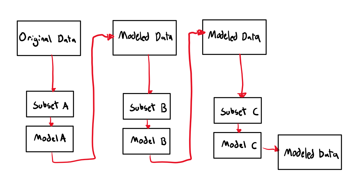
The Boosting algorithm is a type of ensemble learning algorithm that works by training weak models sequentially. First, a model is built from the training data. Then an additional model is built which tries to correct the errors present in the first model. When an input is misclassified by a model, its weight is increased so that next model is more likely to classify it correctly. This procedure is continued and models are added until either the complete training data set is predicted correctly or the maximum number of n models are added.
It works step-by-step like this:
A subset is created from the original dataset, where initially all the data points are given equal weights.
A base model is created on this subset which is used to make predictions on the whole dataset.
Errors are calculated by comparing the actual values vs. the predicted values. The observations that are incorrectly predicted, are given higher weights.
An additional model is created and predictions are made on the dataset, trying to correct the errors of the previous model
The cycle will repeat until the maximum number of n models are added.
The final model (strong model) is the weighted mean of all the models (weak model).
Visualization on how the boosting algorithm works
10.6.3.1 Example: AdaBoost
The AdaBoost algorithm, which is short for “Adaptive Boosting,” was one of the first boosting methods that saw an increase in accuracy and speed performance of models. AdaBoost focuses on enhnacement in performance in areas where the first iteration of the model fails.
We can see an implmentation of this algorithm below:
The AdaBoostClassifier method has some of the following parameters:
estimator - this parameter takes the algoithm we want to use, in this example we use the DecisionTreeClassifier for our weak learners.
n_estimators - this parameter takes the amount of weak learners we want to use.
learning_rate - this parameter learning rate reduces the contribution of the classifier by this value. It has a default value of 1.
random_state - Seed used by the random number generator so we can reproduce out results.
XGBoost is widely considered as one of the most important boosting methods for its advantages over other boosting algorithms.
Other boosting algorithms typically use gradiant descent to find the minima of the n features mapped in n dimensional space. However, XGBoost instead uses the a mathematical technique called the Newton–Raphson method which uses the second derivative of the function which provides curvature information in contract to algorithms using gradiant descent which only use the first derivative.
XGBoost has its own python library called xgboost just to itself for which we wrote the example code below.
The XGBClassifer contains some of the following parameters:
learning_rate - this parameter takes the amount of weak learners we want to use.
random_state - Random number seed.
importance_type - The feature to focus on; either gain, weight, cover, total_gain or total_cover.
from xgboost import XGBClassifierxgboost = XGBClassifier( n_estimators =1000, learning_rate =0.05, random_state =0)xgboost.fit(X_train, y_train)score_xgb = xgboost.score(X_test,y_test)print("Accuracy Score for XGBoost Classifier: "+str(score_xgb))
Accuracy Score for XGBoost Classifier: 0.836
10.6.4 Comparison
Now with all that being said, which should you use? Bagging or Boosting?
Both Bagging and Boosting combine several estimates from different models so both will turn out a model with higher stability.
If you find that the problem when using a single model gets a high error, bagging will rarely be better but on the other hand boosting will generate a combined model with lower errors.
Conversely, if your single model is over-fitting then typically bagging is the best option and boosting will not help for over-fitting. Therefore, bagging iw what you want.
10.6.4.1 Similarites
Below is a set of similarites between Bagging and Boosting:
Both are ensemble learning methods to get N models all from one individual model
Both use random sampling to generate several random subsets
Both make the final decision by averaging and combining the N learners (or taking the majority of them i.e Majority Voting).
Both reduce variance and provide higher data stability than one individual model would.
10.6.4.2 Differences:
Below is a set of differences between Bagging and Boosting:
Bagging combines predictions belonging to the same type while boosting is a way of combining predictions that belong to different types
Bagging decreases variance while boosting decreases bias. If the classifier is unstable (high variance), then we using Bagging. If the classifier is stable and simple (high bias), then we should use Boosting.
Bagging each model receives equal weight where in Boosting each model is weighted based on their performance.
Bagging has models run in parallel, independent of one another while Boosting has them run sequentially so each model is dependent on the previous
In Bagging different training data subsets are randomly generated with replacement segemnts of the original training dataset. In Boosting each new subsets contains the elements that were misclassified by previous models.
Bagging attempts to solve over-fitting problem while Boosting does not.
10.6.4.3 Conclusion:
We have explained what an ensemble method is and how Bagging and Boosting algorithms function.
We have demonstrated the differences and similaries between the two ensemble methods: Bagging and Boosting.
We showed how to implement both Bagging and Boosting algorithms into Python
Naive Bayes classifiers are based on Bayesian classification methods that are derived from Bayes’s theorem. This theorem is an equation that describes the relationship between the conditional probabilities of statistical quantities. In Bayesian classification, the objective is to find the probability of a label given a set of observed features. Bayes’s theorem enables us to express this in terms of more computationally feasible quantities.
The “naive” part of Naive Bayes comes from the assumption of independence between features, which is a simplifying assumption that allows for efficient computation and makes the algorithm particularly well-suited for high-dimensional data. However, this assumption may not hold true in all cases, and there are variants of Naive Bayes that relax this assumption. These classifiers are most commonly used in fields such as natural language processing, image recognition, and spam filtering.
10.7.1.0.1 Installation
Naive Bayes classifiers are found in scikit-learn
pip install scikit-learn
10.7.1.0.2 Types of Naive Bayes classifiers
There are three main types of Naive Bayes classifiers:
Gaussian Naive Bayes - used for continuous input variables that are normally distributed
Multinomial Naive Bayes - used for discrete input variables such as text
Bernoulli Naive Bayes - used for binary input variables such as spam detection
10.7.2 Gaussian Naive Bayes
Gaussian Naive Bayes is possibly the simplest of the three, with the assumption being that data from each label is drawn from a simple Gaussian distribution. In doing this, all the model needs for prediction is the mean and standard deviation of each target’s distribution.
Before getting into anything, we need to load all the necessary packages, including those outside of sklearn.
load_iris is a dataset available from sklearn to use for classification testing.
import pandas as pdimport numpy as npimport seaborn as snsimport matplotlib.pyplot as pltfrom sklearn.datasets import load_irisfrom sklearn.model_selection import train_test_splitfrom sklearn.naive_bayes import GaussianNBfrom sklearn.metrics import accuracy_score, confusion_matrix
First, we load the iris dataset, transform it into a pandas dataframe, adjust labels and preview the data
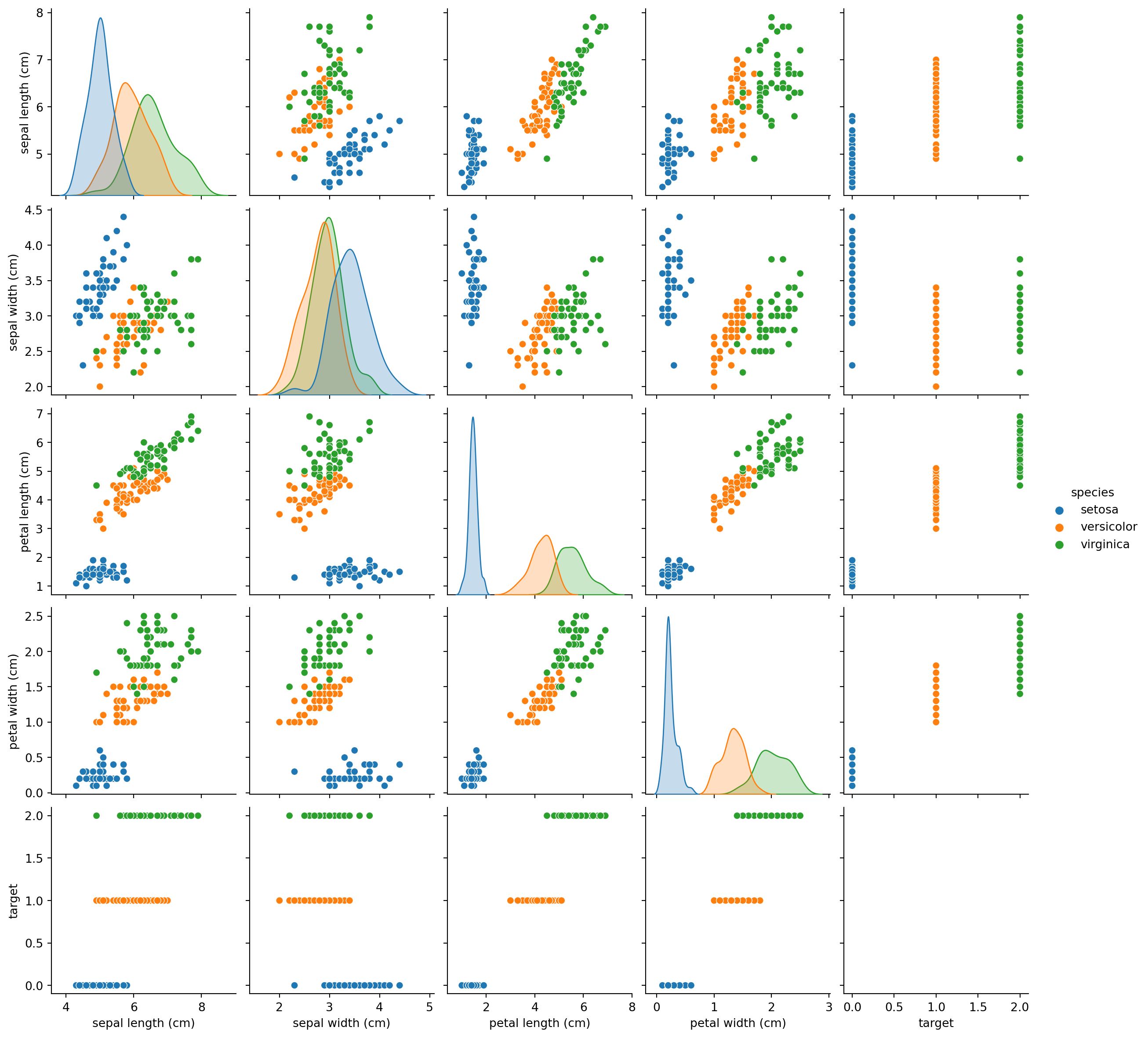
We plot the data using a pairplot to visualize the relationships between the features
sns.pairplot(df, hue="species")plt.show()
As we can see, certain variables graphed against one another show distinct clusters. GaussianNB() accounts for these, and utilizes these distinctions in classification.
Split the data into training and testing sets before calling GaussianNB() and fitting the data.
In a Jupyter environment, please rerun this cell to show the HTML representation or trust the notebook. On GitHub, the HTML representation is unable to render, please try loading this page with nbviewer.org.
GaussianNB()
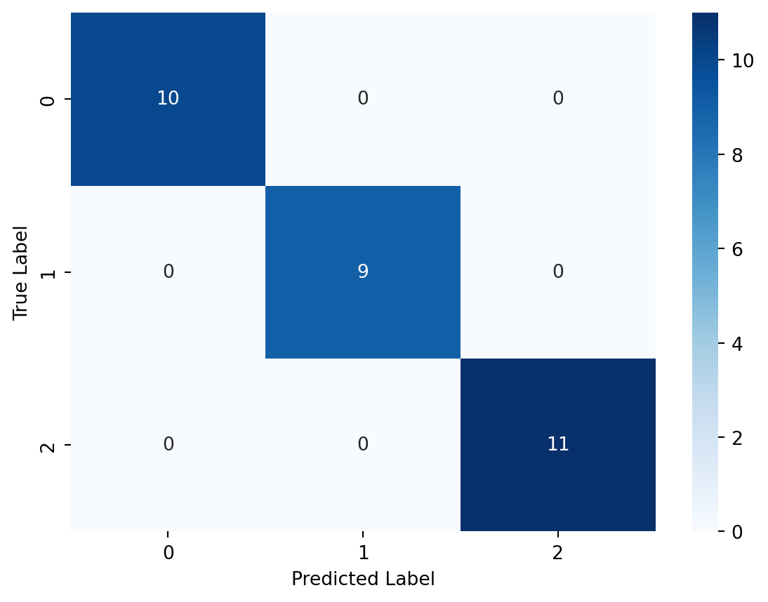
We then create y_pred, evaluate the accuracy of the model, and view the confusion matrix.
This data is meant for displaying classification methods, so it is no surprise that our model is perfect. In general, however, dealing with data that has plenty of targets/labels can be perfect for Gaussian Naive Bayes, as in these instances, the assumptions of independence become less detrimental.
10.7.3 Multinomial Naive Bayes Classifiers
Along with Gaussian Naive Bayes, Multinomial Naive Bayes operates off of the assumption that the features are generated from a simple multinomial distribution.
Multinomial Naive Bayes is well-suited for features that represent counts or count rates since the multinomial distribution models the probability of observing counts across multiple categories.
10.7.3.0.1 Text Classification
One of the best uses for this is in text classification, as it deals with counts/frequencies of words.
To start this example, we load a dataset from sklearn, along with MultinomialNB. CountVectorizer is also loaded, as we are no longer dealing with numerical data.
from sklearn.datasets import fetch_20newsgroupsfrom sklearn.feature_extraction.text import CountVectorizerfrom sklearn.naive_bayes import MultinomialNB
This example will use the fetch_20newsgroups dataset, which is a collection of newsgroup posts on various topics. Now we split it into a training set and a test set.
We can also preview the data, and see the target names, data, and targets
['alt.atheism', 'comp.graphics', 'comp.os.ms-windows.misc', 'comp.sys.ibm.pc.hardware', 'comp.sys.mac.hardware', 'comp.windows.x', 'misc.forsale', 'rec.autos', 'rec.motorcycles', 'rec.sport.baseball', 'rec.sport.hockey', 'sci.crypt', 'sci.electronics', 'sci.med', 'sci.space', 'soc.religion.christian', 'talk.politics.guns', 'talk.politics.mideast', 'talk.politics.misc', 'talk.religion.misc']
From: lerxst@wam.umd.edu (where's my thing)
Subject: WHAT car is this!?
Nntp-Posting-Host: rac3.wam.umd.edu
Organization: University of Maryland, College Park
Lines: 15

 I was wondering if anyone out there could enlighten me on this car I saw
the other day. It was a 2-door sports car, looked to be from the late 60s/
early 70s. It was called a Bricklin. The doors were really small. In addition,
the front bumper was separate from the rest of the body. This is
all I know. If anyone can tellme a model name, engine specs, years
of production, where this car is made, history, or whatever info you
have on this funky looking car, please e-mail.

Thanks,
- IL
   ---- brought to you by your neighborhood Lerxst ----


7
Here we get an idea of our targets, as well as one data example and the target it belongs to.
We then preprocess the data, converting categorical data to numerical.
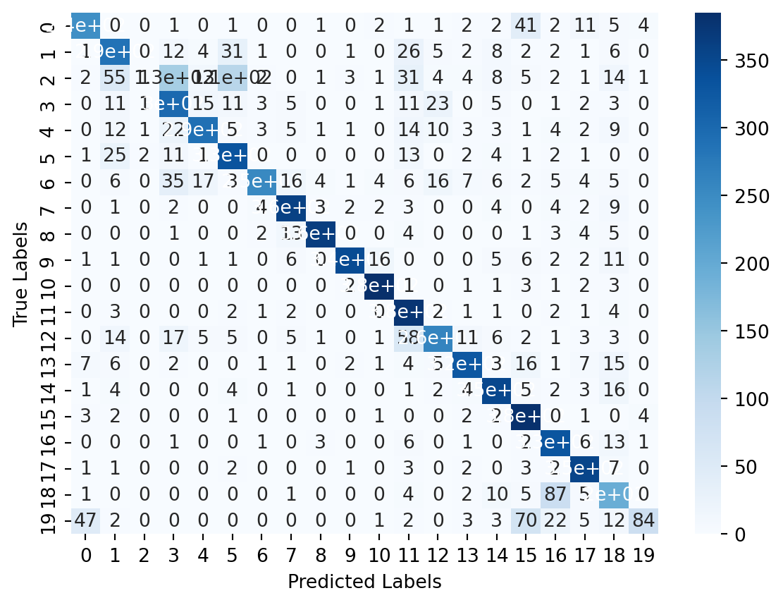
The true labels are shown on the y-axis and the predicted labels are shown on the x-axis. The cells of the heatmap show the number of test instances that belong to a particular class (true label) and were classified as another class (predicted label).
10.7.4 Complement Naive Bayes
Often in cases of imbalanced datasets where certain targets have more data, ComplementNB is used to provide balance to the targets with less data. First we should view our targets.
Our data is fairly balanced here, so ComplementNB may not be necessary.
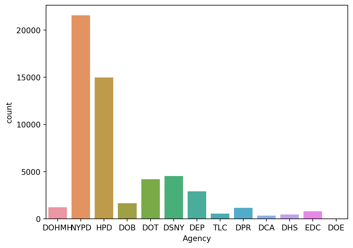
However, using the nyc311 data from the midterm, we can see that the frequency of values by Agency is very imbalanced.
from sklearn.naive_bayes import ComplementNBnyc = pd.read_csv('data/nyc311_011523-012123_by022023.csv')nyc = nyc[['Descriptor', 'Agency']]sns.countplot(x='Agency', data=nyc)plt.show()
As we can see, the NYPD skews the data. We can try using this Naive Bayes classifier to predict what agency a call was made to based on the description.
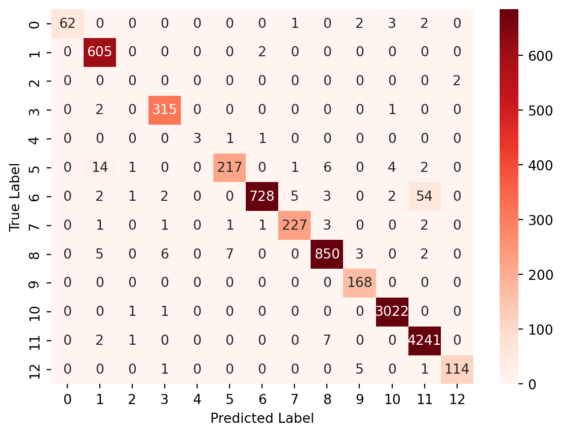
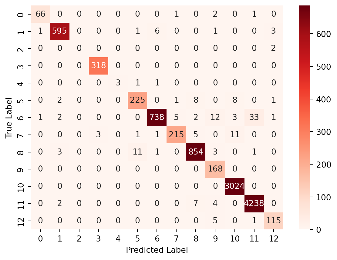
We once again convert the data to vectors, fit our model and evaluate the accuracy/ confusion matrix
It appears that the Multinomial model actually has a higher accuracy; however, if we look a bit closer, we can see that the ComplementNB model indeed does a better job of classifying targets with less data in some cases. For instance, labels 1 and 5 are more accurate. However, it is not true for all labels, and often is slightly less accurate in classification. The use of ComplementNB is a matter of personal judgement / trial and error.
10.7.5 Bernoulli Naive Bayes
Unlike the Multinomial Naive Bayes algorithm, which works with count-based features, Bernoulli Naive Bayes operates on binary features. This makes it particularly well-suited for modeling the presence or absence of certain words or phrases in a document, and makes is especially useful with spam detection. Each feature is assumed to be conditionally independent of all the other features given the class label.
Obviously, our model has some shortcomings. Namely, the accuracy is not great, and it has a high quantity of false negatives. That can partially be attributed to the variable we used, as there is not a lot of distinctions that can be made within the text for factors of each crash. With that being said, for a baseline, it is not bad, and with some tuning and more diverse, larger data to work with, it could classify injuries much better.
10.7.6 Conclusion
In conclusion, using Naive Bayes as a means of classification does have its benefits and shortcomings.
Pros:
Efficiency
Interpretability
Few parameters
Cons:
Simplicity
Data does not always match the assumptions
Few parameters
Overall, Naive Bayes classifiers are best used in finding a solid baseline to build off of.
Vanderplas, Jake. Python Data Science Handbook: Essential Tools for Working with Data. O’REILLY MEDIA, 2023.
10.8 Multiclass Classification with Softmax Regression (by Giovanni Lunetta)
A multiclass classification problem is a type of supervised learning problem in machine learning, where the goal is to predict the class or category of an input observation, based on a set of known classes. In a multiclass classification problem, there are more than two possible classes, and the algorithm must determine which of the possible classes the input observation belongs to.
For example, if we want to classify images of animals into different categories, such as dogs, cats, and horses, we have a multiclass classification problem. In this case, the algorithm must learn to distinguish between the different features of each animal to correctly identify its class.
Multiclass classification problems can be solved using various algorithms, such as logistic regression, decision trees, support vector machines, and neural networks. The performance of these algorithms is typically evaluated using metrics such as accuracy, precision, recall, and F1 score.
10.8.1 Softmax Regression?
Softmax regression is a type of logistic regression that is often used for multiclass classification problems. In a multiclass classification problem, the goal is to predict the class of an input observation from a set of possible classes. Softmax regression provides a way to model the probabilities of the input observation belonging to each of the possible classes.
In softmax regression, the model’s output is a vector of probabilities that represent the likelihood of the input observation belonging to each of the possible classes. The softmax function is used to map the output of the linear regression model to a probability distribution over the classes, ensuring that the probabilities of all classes sum to one.
The goal of softmax regression is to predict the probability of an input observation belonging to each of the possible classes. To achieve this, we compute the weighted sum of the input features \(\vec{x}\) with a weight vector \(\vec{w}_j\) for each class \(j\), and add a bias term \(b_j\). This gives us a scalar value \(z_j\) for each class \(j\). We then apply the softmax function to the \(z\) values to obtain a probability distribution over the possible classes.
More specifically, for a given input observation, we compute the scalar values \(z_j\) for all \(N\) classes as follows: \[
z_j = \vec{w}_j \cdot \vec{x} + b_j,\ \forall j \in {1, 2, \ldots, N}
\] Or, in our example: \[
z_1 = \vec{w}_1 \cdot \vec{x} + b_1
\]\[
z_2 = \vec{w}_2 \cdot \vec{x} + b_2
\]\[
z_3 = \vec{w}_3 \cdot \vec{x} + b_3
\]
The equations provided describe how the model computes a set of scores for each class, which are used to compute the probability distribution over the classes.
Each of the equations describes a linear regression model that computes a score, \(z_i\), for class \(i\) based on the input vector \(\vec{x}\) and a set of weights, \(\vec{w}_i\), and bias, \(b_i\).
Scores refer to the scalar values \(z_j\) computed for each class \(j\). These scores represent the model’s confidence in the input observation belonging to each of the possible classes, and are used to compute the final probability distribution over the classes.
For example, if we have three classes (1, 2, and 3), and the model computes scores of 0.7, 0.2, and 0.1 for each class respectively, this would indicate that the model is most confident that the input observation belongs to class 1, but has lower confidence that it belongs to classes 2 and 3. The probabilities computed from these scores would reflect this relative confidence as well.
Let’s break down the first equation in the example:
\[z_1 = \vec{w}_1 \cdot \vec{x} + b_1\]
Here, \(\vec{w}_1\) is a vector of weights that corresponds to the input features. Each weight represents the importance of a feature in determining the score for class 1. The dot product of the weight vector and input vector, \(\vec{w}_1 \cdot \vec{x}\), is a weighted sum of the input features that determines the contribution of each feature to the score. The bias term, \(b_1\), represents a constant offset that can be used to shift the scores for class 1 up or down.
The scores for classes 2 and 3 are computed using similar equations, but with different weight vectors and biases. The scores can be positive or negative, depending on the input features and the weight values. The sign and magnitude of the scores determine which classes are more likely to be predicted by the model.
To convert the scores to a probability distribution over the classes, the model uses the softmax function, which takes the exponent of each score and normalizes them to sum up to 1. The softmax function outputs a vector of probabilities, where each element represents the probability of the input belonging to a specific class. \[
a_j = \frac{e^{z_j}}{\sum\limits_{k=1}^N e^{z_k}} = P(y=j \mid \vec{x})
\]
In softmax regression, the cost function is used to measure how well the model predicts the probability of an input belonging to each of the possible classes. The goal is to find the set of weights and biases that minimize the cost function, which measures the difference between the predicted probabilities and the true labels.
The cross-entropy loss is a commonly used cost function for softmax regression. The cross-entropy loss is a measure of the dissimilarity between the predicted probability distribution and the true probability distribution. The cross-entropy loss is given by the following two identical formulas: \[
J(\vec{w},b) = -\frac{1}{N}\sum_{i=1}^{N}\sum_{j=1}^{k}y_{ij}\log(\hat{y}_{ij})
\] where \(\hat{y}_{ij}\) is the predicted probability of example \(i\) belonging to class \(j\)\[
\text{loss}(a_1, a_2, \dots, a_n, y) =
\begin{cases}
-\log(a_1) & \text{if } y = 1 \\
-\log(a_2) & \text{if } y = 2 \\
\vdots & \vdots \\
-\log(a_n) & \text{if } y = n
\end{cases}
\]
Using our example: \[
\text{loss}(a_1, a_2, a_3, y) = \begin{cases}
-\log(a_1) & \text{if } y = 1 \\
-\log(a_2) & \text{if } y = 2 \\
-\log(a_3) & \text{if } y = 3
\end{cases}
\] where \(n\) is the number of training examples, \(k\) is the number of possible classes, \(y_{ij}\) is the true label for example \(i\) and class \(j\), and \(\hat{y}_{ij}\) is the predicted probability for example \(i\) and class \(j\).
The cross-entropy loss can be interpreted as the average number of bits needed to represent the true distribution of the classes given the predicted distribution. A lower cross-entropy loss indicates that the predicted probabilities are closer to the true probabilities.
During training, the model adjusts the weights and biases to minimize the cross-entropy loss. This is typically done using an optimization algorithm such as gradient descent. The gradient of the cost function with respect to the weights and biases is computed, and the weights and biases are updated in the direction of the negative gradient to reduce the cost.
In summary, the cost function in softmax regression measures the difference between the predicted probability distribution and the true label distribution, and is used to train the model to make better predictions by adjusting the weights and biases to minimize the cost.
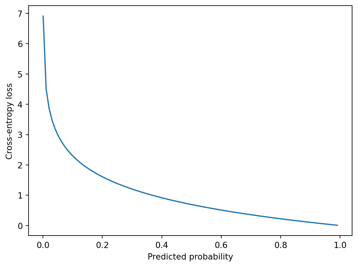
import matplotlib.pyplot as pltimport numpy as np# Define the range of values for the predicted probabilityy_hat = np.arange(0.001, 1.0, 0.01)# Define the true label as 1 for this exampley_true =1# Compute the cross-entropy loss for each value of y_hatloss =- y_true * np.log(y_hat) - (1- y_true) * np.log(1- y_hat)# Plot the loss functionplt.plot(y_hat, loss)plt.xlabel('Predicted probability')plt.ylabel('Cross-entropy loss')plt.show()
In this example, we define a range of values for the predicted probability, y_hat, and set the true label to 1 for simplicity. We then compute the cross-entropy loss for each value of y_hat using the formula for the cross-entropy loss. Finally, we plot the loss function as a function of the predicted probability.
The resulting plot should show a U-shaped curve, with the minimum value of the loss occurring at a predicted probability of 1.0 for the true class and 0.0 for the other class.
The U-shaped curve of the cross-entropy loss function is a reflection of the way the loss function penalizes incorrect predictions. The intuition behind this shape is as follows:
If the model correctly predicts the probability of the true class to be 1.0 (i.e., the predicted probability distribution perfectly matches the true label distribution), then the loss function evaluates to 0.0. This is the minimum possible value of the loss function, and corresponds to the best possible prediction.
As the predicted probability of the true class decreases from 1.0, the loss function begins to increase. This reflects the increasing penalty for incorrectly predicting the probability of the true class.
As the predicted probability of the true class approaches 0.0, the loss function increases very rapidly. This reflects the fact that the model is very confident in an incorrect prediction, and the penalty for this kind of error is very high.
Similarly, as the predicted probability of the true class approaches 1.0 from below, the loss function increases very rapidly again. This reflects the fact that the model is not confident enough in the correct prediction, and the penalty for this kind of error is also very high.
Finally, as the predicted probability of the true class approaches 1.0 from above, the loss function begins to increase more slowly again. This reflects the fact that the model is becoming more confident in the correct prediction, and the penalty for being slightly off is lower than for being very wrong.
Overall, the U-shaped curve of the cross-entropy loss function reflects the way that the model is penalized for incorrect predictions. The loss function is high when the model is very confident in an incorrect prediction, or not confident enough in a correct prediction, and is low when the model makes a perfect prediction.
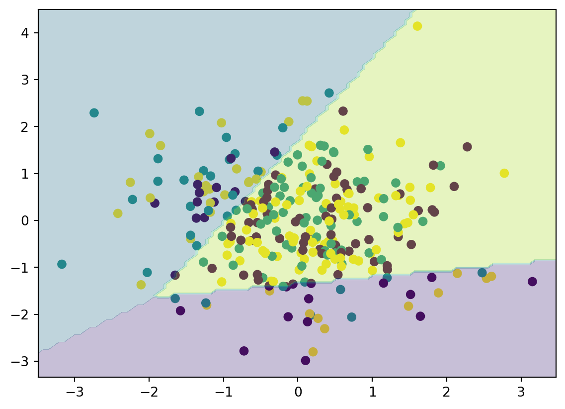
This code generates a scatter plot of the data points, with each class represented by a different color. It then plots the decision boundaries of the classifier, which are represented by the colored regions. The regions are created by classifying a large grid of points that spans the plot, and then plotting the regions of the grid that correspond to each class.
10.9 Synthetic Minority Oversampling Technique
Sythetic Minority Oversampling TEchnique (SMOTE) is an approach for classification with imbalanced datasets (Chawla et al. 2002). A dataset is imbalanced if the classification categories are not approximately equally represented. For example, in rare disease diagnosis or fraud detection, the diseased or fraud cases are much less frequent than the “normal” cases. Further, the cost of misclassifying an abnormal (interesting) case as a normal case is often much higher than the cost of the reverse error. Under-sampling of the majority (normal) class has been proposed as a good means of increasing the sensitivity of a classifier to the minority class. In a similar way, over-sampling the minority (abnormal) class helps improve the classifier performance too. A combination of over-sampling the minority and under-sampling the majority (normal) class can achieve even better classifier performance.
10.9.1 Introduction
The problem with imbalanced data is that, again, accuracy is not a good metric for performance evaluation. A silly approach that classifies all cases as normal would have high accuracy but is useless.
Undersampling means that you discard a number of data points of the class that is present too often. The disadvantage of undersampling is loss of valuable data (information). It coul dbe effective when there is a lot of data, and the class imbalance is not so large. For extremely imbalanced data, undersampling could result in almost no data.
Oversampling makes duplicates of the data that is the least present in the data. But, wait a minute. We would be creating data that is not real and introducing false information into modeling.
At the end, we need to assess the predictive performance of our model on a non-oversampled data set. After all, out-of-sample predictions will be done on non-oversampled data and therefore this is how we should measure models’ performance.
10.9.2 SMOTE Algorithm
SMOTE is a data augumentation approach that creates synthetic data points based on the original data points. It could be viewed as an advanced version of oversampling, except that instead of making exact duplicates of observations in the less present class, we add small perturbations to the copied data points. Therefore, we are not generating duplicates, but rather creating synthetic data points that are slightly different from the original data points.
How exactly synthetic data point is formed? After a random case is drawn from the minority class, take one of its \(k\)~nearest neighbors, and move the current case slightly in the direction of this neighbor. As a result, the synthetic data point is not an exact copy of an existing data point while being too different from the known observations in the minority class.
The data augumentation influences both precision and recall. Just to refresh, precision measures how many identified items are relevant, while recall measures how many relevant items are identified. SMOTE generally leads to an increase in recall, at the cost of lower precision. That is, it will add more predictions of the minority class: some of them correct (increasing recall), but some of them wrong (decreasing precision). The overall model accuracy may also decrease, but this is not a problem because, again, accuracy is not a good in case of imbalanced data.
# Import the dataimport pandas as pddata = pd.read_csv('https://raw.githubusercontent.com/JoosKorstanje/datasets/main/sales_data.csv')data.head()
time_on_page
pages_viewed
interest_ski
interest_climb
buy
0
282.0
3.0
0
1
1
1
223.0
3.0
0
1
1
2
285.0
3.0
1
1
1
3
250.0
3.0
0
1
1
4
271.0
2.0
1
1
1
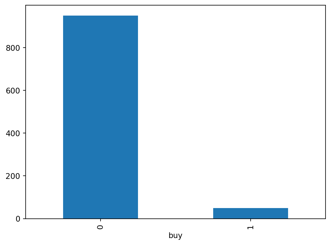
Check the distribution of buyers vs non-buyers.
# Showing the class imbalance between buyers and non-buyersdata.pivot_table(index='buy', aggfunc='size').plot(kind='bar')
<AxesSubplot: xlabel='buy'>
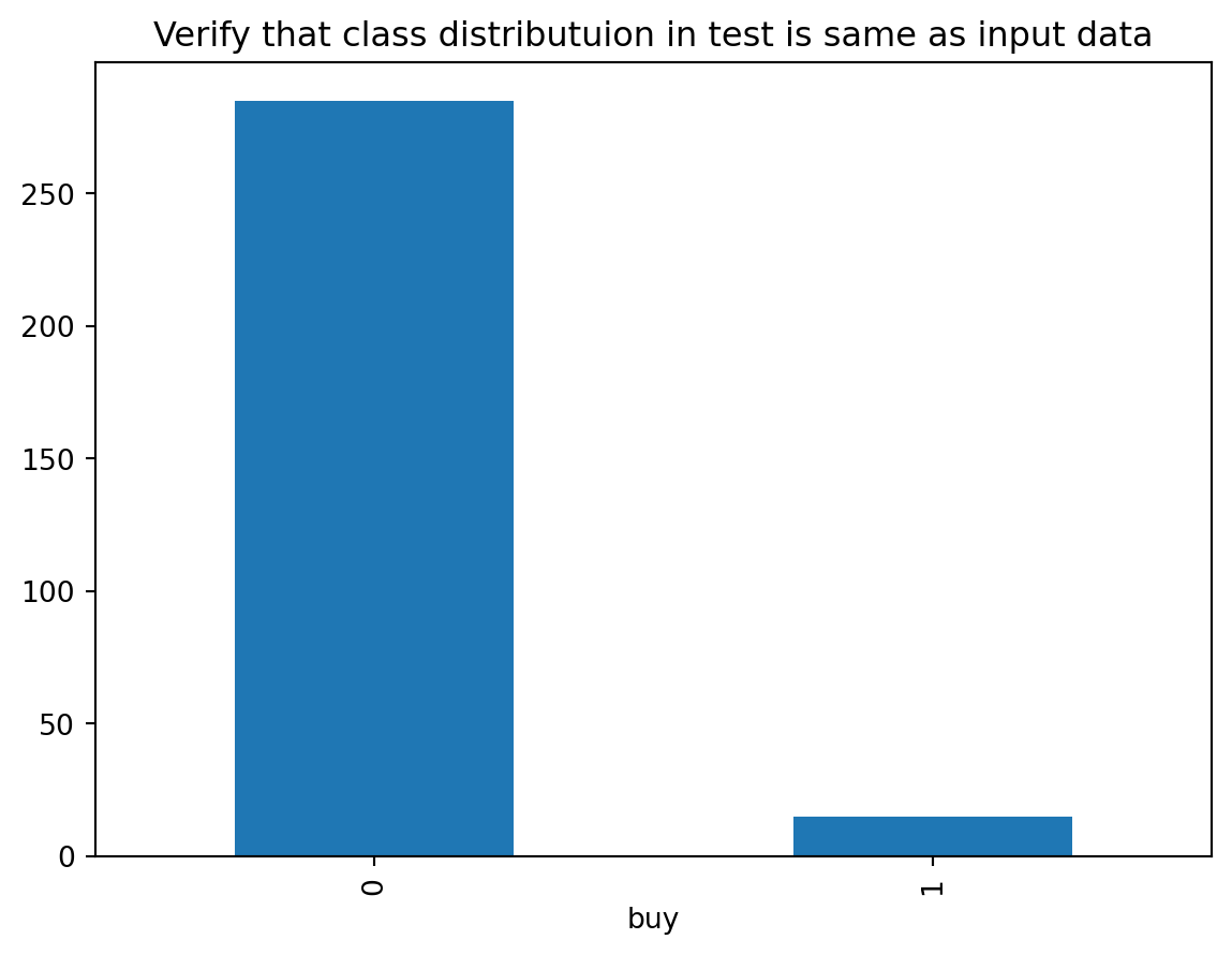
Use stratefied sampling to split the data into training (70%) and testing sets (30%) to avoid ending up with overly few buyers in the testing set.
from sklearn.model_selection import train_test_splittrain, test = train_test_split(data, test_size =0.3, stratify=data.buy)test.pivot_table(index='buy', aggfunc='size').plot(kind='bar', title='Verify that class distributuion in test is same as input data')
<AxesSubplot: title={'center': 'Verify that class distributuion in test is same as input data'}, xlabel='buy'>
Build a logistic regression as benchmark to assess the benefit of SMOTE.
from sklearn.linear_model import LogisticRegression# Instantiate the Logistic Regression with only default settingsmy_log_reg = LogisticRegression()# Fit the logistic regression on the independent variables of the train data with buy as dependent variablemy_log_reg.fit(train[['time_on_page', 'pages_viewed', 'interest_ski', 'interest_climb']], train['buy'])# Make a prediction using our model on the test setpreds = my_log_reg.predict(test[['time_on_page', 'pages_viewed', 'interest_ski', 'interest_climb']])
Obtain the confusion matrix of the benchmark model.
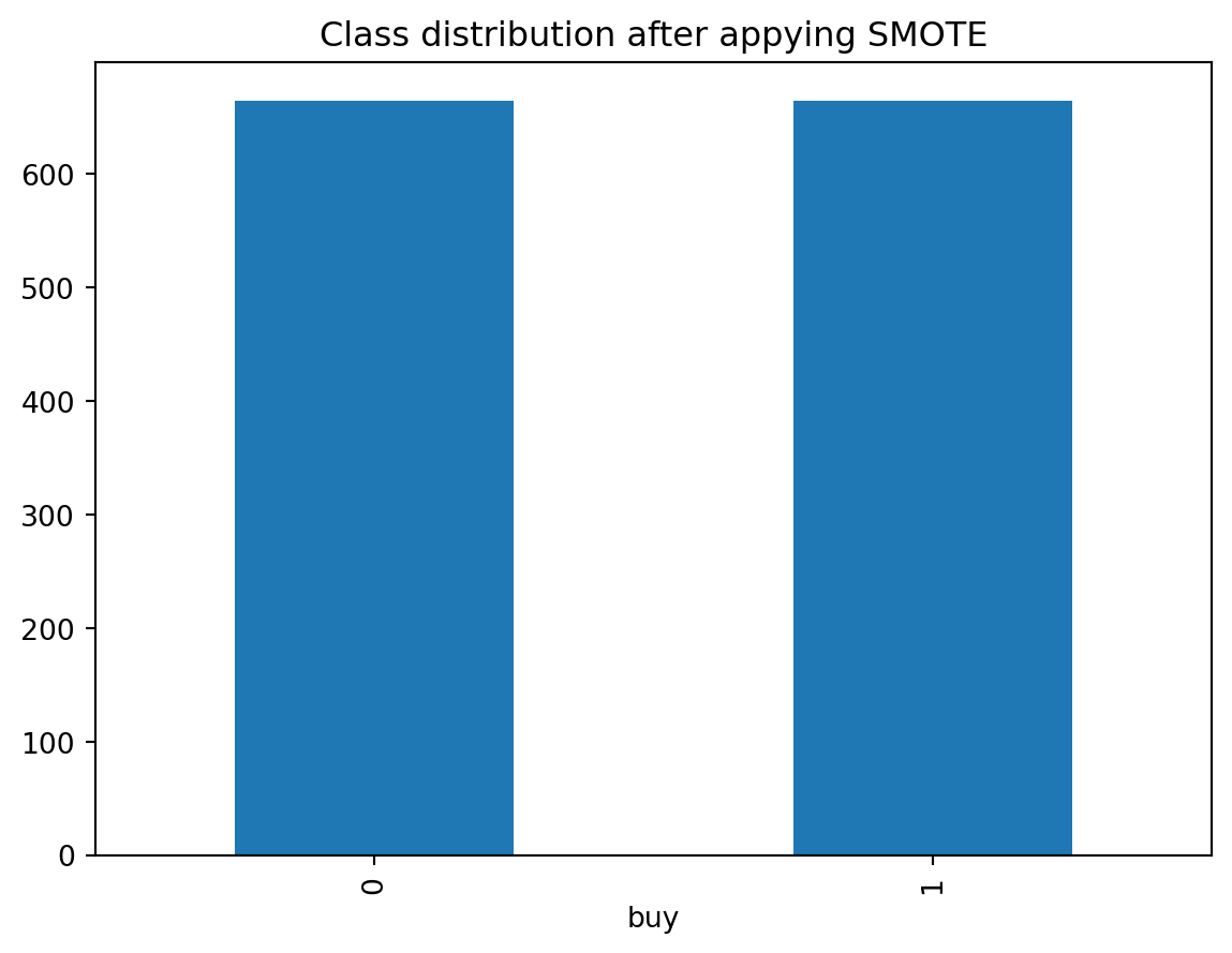
Check the distribution of the buyers and non-buyers
pd.Series(y_resampled).value_counts().plot(kind='bar', title='Class distribution after appying SMOTE', xlabel='buy')
<AxesSubplot: title={'center': 'Class distribution after appying SMOTE'}, xlabel='buy'>
Train the logistic model with SMOTE augmented data.
# Instantiate the new Logistic Regressionlog_reg_2 = LogisticRegression()# Fit the model with the data that has been resampled with SMOTElog_reg_2.fit(X_resampled, y_resampled)# Predict on the test set (not resampled to obtain honest evaluation)preds2 = log_reg_2.predict(test[['time_on_page', 'pages_viewed', 'interest_ski', 'interest_climb']])
What the the changes from the first to the second model? + Recall of nonbuyers went down from 1.00 to 0.90: there are more nonbuyers that we did not succeed to find + Recall of buyers went up from 0.47 to 0.87: we succeeded to identify many more buyers + The precision of buyers went down from 0.88 to 0.32: the cost of correctly identifying more buyers is that we now also incorrectly identify more buyers (identifying visitors as buyers while they are actually nonbuyers)!
We are now better able to find buyers, at the cost of also wrongly classifying more nonbuyers as buyers.
Chawla, Nitesh V, Kevin W Bowyer, Lawrence O Hall, and W Philip Kegelmeyer. 2002. “SMOTE: Synthetic Minority over-Sampling Technique.”Journal of Artificial Intelligence Research 16: 321–57.