import pandas as pd5 Data Manipulation
5.1 Introduction
Data manipulation is crucial for transforming raw data into a more analyzable format, essential for uncovering patterns and ensuring accurate analysis. This chapter introduces the core techniques for data manipulation in Python, utilizing the Pandas library, a cornerstone for data handling within Python’s data science toolkit.
Python’s ecosystem is rich with libraries that facilitate not just data manipulation but comprehensive data analysis. Pandas, in particular, provides extensive functionality for data manipulation tasks including reading, cleaning, transforming, and summarizing data. Using real-world datasets, we will explore how to leverage Python for practical data manipulation tasks.
By the end of this chapter, you will learn to:
- Import/export data from/to diverse sources.
- Clean and preprocess data efficiently.
- Transform and aggregate data to derive insights.
- Merge and concatenate datasets from various origins.
- Analyze real-world datasets using these techniques.
5.2 Data Manipulation with Pandas
This section is prepared by Lang Lang. I am a senior student double majoring in
data science and economics in University of Connecticut.
5.2.1 Introduction
In this section, I will introduce about data manipulation using Pandas,
which is a powerful Python library for working with data. I’ll walk through
some basic operations like filtering, merging, and summarizing data using a real
data set of NYC motor vehicle collisions.
Pandas is a powerful Python library for data manipulation and analysis. It
provides two key data structures:
- Series: A one-dimensional labeled array.
- Data Frame: A two-dimensional labeled table with rows and columns.
5.2.1.1 Why Use Pandas?
- Efficiently handles large data sets.
- Provides flexible data manipulation functions.
- Works well with NumPy and visualization libraries like Matplotlib.
5.2.2 Loading Data
5.2.2.1 Reading NYC Crash Data
We’ll work with the NYC Motor Vehicle Collisions data set in the class notes
repository.
- Using the following code to import the Pandas library in Python
- Using the following code to load the data set
df = pd.read_csv("data/nyccrashes_2024w0630_by20250212.csv")5.2.2.2 Renaming The Columns
Using the following codes to rename the columns.
df.columns = [col.strip().lower().replace(" ", "_") for col in df.columns]
df.columns
Index(['crash_date', 'crash_time', 'borough', 'zip_code', 'latitude',
'longitude', 'location', 'on_street_name', 'cross_street_name',
'off_street_name', 'number_of_persons_injured',
'number_of_persons_killed', 'number_of_pedestrians_injured',
'number_of_pedestrians_killed', 'number_of_cyclist_injured',
'number_of_cyclist_killed', 'number_of_motorist_injured',
'number_of_motorist_killed', 'contributing_factor_vehicle_1',
'contributing_factor_vehicle_2', 'contributing_factor_vehicle_3',
'contributing_factor_vehicle_4', 'contributing_factor_vehicle_5',
'collision_id', 'vehicle_type_code_1', 'vehicle_type_code_2',
'vehicle_type_code_3', 'vehicle_type_code_4', 'vehicle_type_code_5'],
dtype='object')5.2.2.3 Viewing the First Few Rows
The head function in Pandas is used to display the first few rows of a DataFrame.
df.head() # Default value of n is 5| crash_date | crash_time | borough | zip_code | latitude | longitude | location | on_street_name | cross_street_name | off_street_name | ... | contributing_factor_vehicle_2 | contributing_factor_vehicle_3 | contributing_factor_vehicle_4 | contributing_factor_vehicle_5 | collision_id | vehicle_type_code_1 | vehicle_type_code_2 | vehicle_type_code_3 | vehicle_type_code_4 | vehicle_type_code_5 | |
|---|---|---|---|---|---|---|---|---|---|---|---|---|---|---|---|---|---|---|---|---|---|
| 0 | 06/30/2024 | 23:17 | BRONX | 10460.0 | 40.838844 | -73.87817 | (40.838844, -73.87817) | EAST 177 STREET | DEVOE AVENUE | NaN | ... | Unspecified | NaN | NaN | NaN | 4737486 | Sedan | Pick-up Truck | NaN | NaN | NaN |
| 1 | 06/30/2024 | 8:30 | BRONX | 10468.0 | 40.862732 | -73.90333 | (40.862732, -73.90333) | WEST FORDHAM ROAD | GRAND AVENUE | NaN | ... | Unspecified | NaN | NaN | NaN | 4737502 | Sedan | NaN | NaN | NaN | NaN |
| 2 | 06/30/2024 | 20:47 | NaN | NaN | 40.763630 | -73.95330 | (40.76363, -73.9533) | FDR DRIVE | NaN | NaN | ... | NaN | NaN | NaN | NaN | 4737510 | Sedan | NaN | NaN | NaN | NaN |
| 3 | 06/30/2024 | 13:10 | BROOKLYN | 11234.0 | 40.617030 | -73.91989 | (40.61703, -73.91989) | EAST 57 STREET | AVENUE O | NaN | ... | Driver Inattention/Distraction | NaN | NaN | NaN | 4737499 | Sedan | Sedan | NaN | NaN | NaN |
| 4 | 06/30/2024 | 16:42 | NaN | NaN | NaN | NaN | NaN | 33 STREET | ASTORIA BOULEVARD | NaN | ... | Unspecified | NaN | NaN | NaN | 4736925 | Sedan | Station Wagon/Sport Utility Vehicle | NaN | NaN | NaN |
5 rows × 29 columns
5.2.2.4 Checking Dataset Structure
The info function in Pandas provides a summary of a DataFrame, including:
- Number of rows and columns
- Column names and data types
- Number of non-null values per column
- Memory usage
df.info()<class 'pandas.core.frame.DataFrame'>
RangeIndex: 1876 entries, 0 to 1875
Data columns (total 29 columns):
# Column Non-Null Count Dtype
--- ------ -------------- -----
0 crash_date 1876 non-null object
1 crash_time 1876 non-null object
2 borough 1334 non-null object
3 zip_code 1334 non-null float64
4 latitude 1745 non-null float64
5 longitude 1745 non-null float64
6 location 1745 non-null object
7 on_street_name 1330 non-null object
8 cross_street_name 944 non-null object
9 off_street_name 546 non-null object
10 number_of_persons_injured 1876 non-null int64
11 number_of_persons_killed 1876 non-null int64
12 number_of_pedestrians_injured 1876 non-null int64
13 number_of_pedestrians_killed 1876 non-null int64
14 number_of_cyclist_injured 1876 non-null int64
15 number_of_cyclist_killed 1876 non-null int64
16 number_of_motorist_injured 1876 non-null int64
17 number_of_motorist_killed 1876 non-null int64
18 contributing_factor_vehicle_1 1865 non-null object
19 contributing_factor_vehicle_2 1426 non-null object
20 contributing_factor_vehicle_3 174 non-null object
21 contributing_factor_vehicle_4 52 non-null object
22 contributing_factor_vehicle_5 14 non-null object
23 collision_id 1876 non-null int64
24 vehicle_type_code_1 1843 non-null object
25 vehicle_type_code_2 1231 non-null object
26 vehicle_type_code_3 162 non-null object
27 vehicle_type_code_4 48 non-null object
28 vehicle_type_code_5 14 non-null object
dtypes: float64(3), int64(9), object(17)
memory usage: 425.2+ KBThis tells us:
The dataset has 1876 rows and 29 columns.
Data types include float64(3), int64(9), object(17).
There are no missing values in any column.
The dataset consumes 425.2+ KB of memory.
5.2.2.5 Descriptive Statistics
The discribe function provides summary statistics for numerical columns in a
Pandas DataFrame.
df.describe()| zip_code | latitude | longitude | number_of_persons_injured | number_of_persons_killed | number_of_pedestrians_injured | number_of_pedestrians_killed | number_of_cyclist_injured | number_of_cyclist_killed | number_of_motorist_injured | number_of_motorist_killed | collision_id | |
|---|---|---|---|---|---|---|---|---|---|---|---|---|
| count | 1334.000000 | 1745.000000 | 1745.000000 | 1876.000000 | 1876.000000 | 1876.000000 | 1876.000000 | 1876.000000 | 1876.0 | 1876.000000 | 1876.000000 | 1.876000e+03 |
| mean | 10902.185157 | 40.649264 | -73.792754 | 0.616738 | 0.004264 | 0.093284 | 0.002665 | 0.065032 | 0.0 | 0.432836 | 0.001599 | 4.738602e+06 |
| std | 526.984169 | 1.689337 | 3.064378 | 0.915477 | 0.103191 | 0.338369 | 0.095182 | 0.246648 | 0.0 | 0.891003 | 0.039968 | 1.772834e+03 |
| min | 10001.000000 | 0.000000 | -74.237366 | 0.000000 | 0.000000 | 0.000000 | 0.000000 | 0.000000 | 0.0 | 0.000000 | 0.000000 | 4.736561e+06 |
| 25% | 10457.000000 | 40.661804 | -73.968540 | 0.000000 | 0.000000 | 0.000000 | 0.000000 | 0.000000 | 0.0 | 0.000000 | 0.000000 | 4.737667e+06 |
| 50% | 11208.500000 | 40.712696 | -73.922960 | 0.000000 | 0.000000 | 0.000000 | 0.000000 | 0.000000 | 0.0 | 0.000000 | 0.000000 | 4.738258e+06 |
| 75% | 11239.000000 | 40.767690 | -73.869180 | 1.000000 | 0.000000 | 0.000000 | 0.000000 | 0.000000 | 0.0 | 1.000000 | 0.000000 | 4.738886e+06 |
| max | 11694.000000 | 40.907246 | 0.000000 | 11.000000 | 4.000000 | 7.000000 | 4.000000 | 1.000000 | 0.0 | 11.000000 | 1.000000 | 4.765601e+06 |
This provides insights such as:
Total count of entries
Mean, min, and max values
Standard deviation
5.2.3 Selecting and Filtering Data
5.2.3.1 Selecting Specific Columns
Sometimes, we only need certain columns.
In this case, you can use select function.
df_selected = df[['crash_date', 'crash_time', 'borough',
                  'number_of_persons_injured']]
df_selected.head() | crash_date | crash_time | borough | number_of_persons_injured | |
|---|---|---|---|---|
| 0 | 06/30/2024 | 23:17 | BRONX | 0 |
| 1 | 06/30/2024 | 8:30 | BRONX | 0 |
| 2 | 06/30/2024 | 20:47 | NaN | 0 |
| 3 | 06/30/2024 | 13:10 | BROOKLYN | 1 |
| 4 | 06/30/2024 | 16:42 | NaN | 1 |
5.2.3.2 Filtering Data
when you would like to filter certain specific data (e.g., Crashes in 2024-06-30),
you can using the following data to define:
# Convert crash date to datetime format
df['crash_date'] = pd.to_datetime(df['crash_date'])

june30_df = df[df['crash_date'] == '2024-06-30']
june30_df.head()| crash_date | crash_time | borough | zip_code | latitude | longitude | location | on_street_name | cross_street_name | off_street_name | ... | contributing_factor_vehicle_2 | contributing_factor_vehicle_3 | contributing_factor_vehicle_4 | contributing_factor_vehicle_5 | collision_id | vehicle_type_code_1 | vehicle_type_code_2 | vehicle_type_code_3 | vehicle_type_code_4 | vehicle_type_code_5 | |
|---|---|---|---|---|---|---|---|---|---|---|---|---|---|---|---|---|---|---|---|---|---|
| 0 | 2024-06-30 | 23:17 | BRONX | 10460.0 | 40.838844 | -73.87817 | (40.838844, -73.87817) | EAST 177 STREET | DEVOE AVENUE | NaN | ... | Unspecified | NaN | NaN | NaN | 4737486 | Sedan | Pick-up Truck | NaN | NaN | NaN |
| 1 | 2024-06-30 | 8:30 | BRONX | 10468.0 | 40.862732 | -73.90333 | (40.862732, -73.90333) | WEST FORDHAM ROAD | GRAND AVENUE | NaN | ... | Unspecified | NaN | NaN | NaN | 4737502 | Sedan | NaN | NaN | NaN | NaN |
| 2 | 2024-06-30 | 20:47 | NaN | NaN | 40.763630 | -73.95330 | (40.76363, -73.9533) | FDR DRIVE | NaN | NaN | ... | NaN | NaN | NaN | NaN | 4737510 | Sedan | NaN | NaN | NaN | NaN |
| 3 | 2024-06-30 | 13:10 | BROOKLYN | 11234.0 | 40.617030 | -73.91989 | (40.61703, -73.91989) | EAST 57 STREET | AVENUE O | NaN | ... | Driver Inattention/Distraction | NaN | NaN | NaN | 4737499 | Sedan | Sedan | NaN | NaN | NaN |
| 4 | 2024-06-30 | 16:42 | NaN | NaN | NaN | NaN | NaN | 33 STREET | ASTORIA BOULEVARD | NaN | ... | Unspecified | NaN | NaN | NaN | 4736925 | Sedan | Station Wagon/Sport Utility Vehicle | NaN | NaN | NaN |
5 rows × 29 columns
5.2.3.3 Filter A DataFrame
The query function in Pandas is used to filter a DataFrame using a more
readable, SQL-like syntax. For example, now I would like to find the crashes with
the number of persons injured more than 2. We can using the following code:
df_filtered = df.query("`number_of_persons_injured` > 2")
df_filtered.head()| crash_date | crash_time | borough | zip_code | latitude | longitude | location | on_street_name | cross_street_name | off_street_name | ... | contributing_factor_vehicle_2 | contributing_factor_vehicle_3 | contributing_factor_vehicle_4 | contributing_factor_vehicle_5 | collision_id | vehicle_type_code_1 | vehicle_type_code_2 | vehicle_type_code_3 | vehicle_type_code_4 | vehicle_type_code_5 | |
|---|---|---|---|---|---|---|---|---|---|---|---|---|---|---|---|---|---|---|---|---|---|
| 20 | 2024-06-30 | 13:05 | NaN | NaN | 40.797447 | -73.946710 | (40.797447, -73.94671) | MADISON AVENUE | NaN | NaN | ... | Unspecified | NaN | NaN | NaN | 4736750 | Sedan | Station Wagon/Sport Utility Vehicle | NaN | NaN | NaN |
| 33 | 2024-06-30 | 15:30 | BROOKLYN | 11229.0 | 40.610653 | -73.953550 | (40.610653, -73.95355) | KINGS HIGHWAY | OCEAN AVENUE | NaN | ... | NaN | NaN | NaN | NaN | 4737460 | Sedan | NaN | NaN | NaN | NaN |
| 35 | 2024-06-30 | 16:28 | STATEN ISLAND | 10304.0 | 40.589180 | -74.098946 | (40.58918, -74.098946) | JEFFERSON STREET | LIBERTY AVENUE | NaN | ... | Unspecified | NaN | NaN | NaN | 4736985 | Sedan | Sedan | NaN | NaN | NaN |
| 37 | 2024-06-30 | 20:29 | MANHATTAN | 10027.0 | 40.807667 | -73.949290 | (40.807667, -73.94929) | 7 AVENUE | WEST 123 STREET | NaN | ... | Unspecified | NaN | NaN | NaN | 4737257 | Station Wagon/Sport Utility Vehicle | Sedan | NaN | NaN | NaN |
| 45 | 2024-06-30 | 19:56 | BROOKLYN | 11237.0 | 40.709003 | -73.922340 | (40.709003, -73.92234) | SCOTT AVENUE | FLUSHING AVENUE | NaN | ... | Unspecified | Unspecified | NaN | NaN | 4736995 | Sedan | Station Wagon/Sport Utility Vehicle | Moped | NaN | NaN |
5 rows × 29 columns
5.2.4 Merging DataFrames
In Pandas, the merge function is used to combine multiple DataFrames based
on a common column.
This is useful when working with multiple datasets that need to be joined for
analysis.
5.2.4.1 Example: Merging Crash Data with Total Injuries per Borough
Suppose we have a dataset containing crash details, and we want to analyze how
the total number of injuries in each borough relates to individual crashes.
We can achieve this by aggregating the total injuries per borough and merging it
with the crash dataset.
The following code:
Aggregates the total injuries per borough using
.groupby().Selects relevant columns from the main dataset (
collision_id,borough,
number_of_persons_injured).Merges the aggregated injury data with the crash dataset using merge function on
theboroughcolumn.
# Aggregate total injuries per borough
df_borough_info = df.groupby(
          'borough', as_index=False
          )['number_of_persons_injured'].sum()
df_borough_info.rename(
          columns={'number_of_persons_injured': 'total_injuries'},
                  inplace=True)

# Select relevant columns from the main dataset
df_crashes = df[['collision_id', 'borough', 'number_of_persons_injured']]

# Merge crash data with total injuries per borough
df_merged = pd.merge(df_crashes, df_borough_info, on='borough', how='left')

# Display first few rows of the merged dataset
df_merged.head()| collision_id | borough | number_of_persons_injured | total_injuries | |
|---|---|---|---|---|
| 0 | 4737486 | BRONX | 0 | 126.0 |
| 1 | 4737502 | BRONX | 0 | 126.0 |
| 2 | 4737510 | NaN | 0 | NaN |
| 3 | 4737499 | BROOKLYN | 1 | 295.0 |
| 4 | 4736925 | NaN | 1 | NaN |
The merged dataset now includes:
- collision_id: Unique identifier for each crash.
- borough: The borough where the crash occurred.
- number_of_persons_injured: Number of injuries in a specific crash.
- total_injuries: The total number of injuries reported in that borough.
This merged dataset allows us to compare individual crash injuries with the
overall injury trend in each borough, helping in further data analysis and
visualization.
5.2.5 Data Visualization
Visualizing data is crucial to understanding patterns and relationships within
the dataset. In this section, we will create one-variable tables (frequency
table), two-variable tables (contingency table).
5.2.5.1 One-Variable Table
A one-variable table (also called a frequency table) shows the distribution of
values for a single categorical variable.
For example, we can count the number of crashes per borough:
borough_counts = df['borough'].value_counts()
borough_counts
borough
BROOKLYN 462
QUEENS 381
MANHATTAN 228
BRONX 213
STATEN ISLAND 50
Name: count, dtype: int64This table displays the number of accidents recorded in each borough of NYC. It
helps identify which borough has the highest accident frequency.
5.2.5.2 Two-Variable Table
A two-variable table (also called a contingency table) shows the relationship
between two categorical variables.
For example, we can analyze the number of crashes per borough per day:
# make pivot table
borough_day_table = df.pivot_table(
    index='crash_date',
    columns='borough',
    values='collision_id',
    aggfunc='count'
)
borough_day_table| borough | BRONX | BROOKLYN | MANHATTAN | QUEENS | STATEN ISLAND |
|---|---|---|---|---|---|
| crash_date | |||||
| 2024-06-30 | 24 | 69 | 40 | 40 | 8 |
| 2024-07-01 | 27 | 62 | 35 | 45 | 3 |
| 2024-07-02 | 19 | 53 | 37 | 54 | 8 |
| 2024-07-03 | 33 | 59 | 25 | 58 | 3 |
| 2024-07-04 | 27 | 47 | 31 | 44 | 8 |
| 2024-07-05 | 32 | 64 | 28 | 58 | 9 |
| 2024-07-06 | 27 | 62 | 16 | 37 | 6 |
| 2024-07-07 | 24 | 46 | 16 | 45 | 5 |
This table shows the number of accidents per borough for each day in the dataset.
5.2.6 Data Cleaning and Transformation
This part is from the textbook “Python for Data Analysis: Data Wrangling with
Pandas, NumPy, and IPython.” Chapter 5, Third Edition by Wes McK- inney, O’Reilly
Media, 2022. https://wesmckinney.com/book/.
5.2.6.1 Changing Data Types
The following functions in Pandas are used to convert data types. This is
important when working with dates and categorical data to ensure proper analysis.
For example, we want to:
# Convert crash date to datetime format
df['crash_date'] = pd.to_datetime(df['crash_date'])
df['crash_date']

# Convert ZIP code to string
df['zip_code'] = df['zip_code'].astype(str)
df['zip_code']
0 10460.0
1 10468.0
2 nan
3 11234.0
4 nan
...
1871 nan
1872 nan
1873 10468.0
1874 nan
1875 nan
Name: zip_code, Length: 1876, dtype: object5.2.6.2 Sorting Data
We can sort data by one or more columns:
# Sort by date and time
df_sorted = df.sort_values(
    by=['crash_date', 'crash_time'],
    ascending=[True, True]
)
df_sorted.head()| crash_date | crash_time | borough | zip_code | latitude | longitude | location | on_street_name | cross_street_name | off_street_name | ... | contributing_factor_vehicle_2 | contributing_factor_vehicle_3 | contributing_factor_vehicle_4 | contributing_factor_vehicle_5 | collision_id | vehicle_type_code_1 | vehicle_type_code_2 | vehicle_type_code_3 | vehicle_type_code_4 | vehicle_type_code_5 | |
|---|---|---|---|---|---|---|---|---|---|---|---|---|---|---|---|---|---|---|---|---|---|
| 90 | 2024-06-30 | 0:00 | NaN | nan | 40.638268 | -74.07880 | (40.638268, -74.0788) | VICTORY BOULEVARD | NaN | NaN | ... | NaN | NaN | NaN | NaN | 4737312 | Pick-up Truck | NaN | NaN | NaN | NaN |
| 180 | 2024-06-30 | 0:00 | MANHATTAN | 10004.0 | 40.704834 | -74.01658 | (40.704834, -74.01658) | NaN | NaN | 17 BATTERY PLACE | ... | Unspecified | NaN | NaN | NaN | 4737900 | Taxi | Sedan | NaN | NaN | NaN |
| 188 | 2024-06-30 | 0:00 | BRONX | 10455.0 | 40.815754 | -73.89529 | (40.815754, -73.89529) | LONGWOOD AVENUE | BRUCKNER BOULEVARD | NaN | ... | Unspecified | NaN | NaN | NaN | 4737875 | Sedan | Sedan | NaN | NaN | NaN |
| 248 | 2024-06-30 | 0:04 | NaN | nan | 40.712490 | -73.96854 | (40.71249, -73.96854) | WILLIAMSBURG BRIDGE | NaN | NaN | ... | NaN | NaN | NaN | NaN | 4737093 | Bike | NaN | NaN | NaN | NaN |
| 137 | 2024-06-30 | 0:05 | NaN | nan | 40.793980 | -73.97229 | (40.79398, -73.97229) | BROADWAY | NaN | NaN | ... | Unspecified | NaN | NaN | NaN | 4736952 | Sedan | Bike | NaN | NaN | NaN |
5 rows × 29 columns
Now you can see the data is sorted by crash time.
5.2.6.3 Handling Missing Data
Pandas provides methods for handling missing values.
For example, you can using the following codes to fix the missing data.
# Check for missing values
df.isna().sum()
crash_date 0
crash_time 0
borough 542
zip_code 0
latitude 131
longitude 131
location 131
on_street_name 546
cross_street_name 932
off_street_name 1330
number_of_persons_injured 0
number_of_persons_killed 0
number_of_pedestrians_injured 0
number_of_pedestrians_killed 0
number_of_cyclist_injured 0
number_of_cyclist_killed 0
number_of_motorist_injured 0
number_of_motorist_killed 0
contributing_factor_vehicle_1 11
contributing_factor_vehicle_2 450
contributing_factor_vehicle_3 1702
contributing_factor_vehicle_4 1824
contributing_factor_vehicle_5 1862
collision_id 0
vehicle_type_code_1 33
vehicle_type_code_2 645
vehicle_type_code_3 1714
vehicle_type_code_4 1828
vehicle_type_code_5 1862
dtype: int64# Fill missing values with NaN
df.fillna(float('nan'), inplace=True)
df.fillna<bound method NDFrame.fillna of crash_date crash_time borough zip_code latitude longitude \
0 2024-06-30 23:17 BRONX 10460.0 40.838844 -73.878170
1 2024-06-30 8:30 BRONX 10468.0 40.862732 -73.903330
2 2024-06-30 20:47 NaN nan 40.763630 -73.953300
3 2024-06-30 13:10 BROOKLYN 11234.0 40.617030 -73.919890
4 2024-06-30 16:42 NaN nan NaN NaN
... ... ... ... ... ... ...
1871 2024-07-07 20:15 NaN nan 40.677982 -73.791214
1872 2024-07-07 14:45 NaN nan 40.843822 -73.927500
1873 2024-07-07 14:12 BRONX 10468.0 40.861084 -73.911490
1874 2024-07-07 1:40 NaN nan 40.813114 -73.931470
1875 2024-07-07 19:00 NaN nan 40.680960 -73.773575
location on_street_name cross_street_name \
0 (40.838844, -73.87817) EAST 177 STREET DEVOE AVENUE
1 (40.862732, -73.90333) WEST FORDHAM ROAD GRAND AVENUE
2 (40.76363, -73.9533) FDR DRIVE NaN
3 (40.61703, -73.91989) EAST 57 STREET AVENUE O
4 NaN 33 STREET ASTORIA BOULEVARD
... ... ... ...
1871 (40.677982, -73.791214) SUTPHIN BOULEVARD 120 AVENUE
1872 (40.843822, -73.9275) MAJOR DEEGAN EXPRESSWAY NaN
1873 (40.861084, -73.91149) NaN NaN
1874 (40.813114, -73.93147) MAJOR DEEGAN EXPRESSWAY NaN
1875 (40.68096, -73.773575) MARSDEN STREET NaN
off_street_name ... contributing_factor_vehicle_2 \
0 NaN ... Unspecified
1 NaN ... Unspecified
2 NaN ... NaN
3 NaN ... Driver Inattention/Distraction
4 NaN ... Unspecified
... ... ... ...
1871 NaN ... Unspecified
1872 NaN ... Unspecified
1873 2258 HAMPDEN PLACE ... NaN
1874 NaN ... Unspecified
1875 NaN ... NaN
contributing_factor_vehicle_3 contributing_factor_vehicle_4 \
0 NaN NaN
1 NaN NaN
2 NaN NaN
3 NaN NaN
4 NaN NaN
... ... ...
1871 NaN NaN
1872 NaN NaN
1873 NaN NaN
1874 NaN NaN
1875 NaN NaN
contributing_factor_vehicle_5 collision_id vehicle_type_code_1 \
0 NaN 4737486 Sedan
1 NaN 4737502 Sedan
2 NaN 4737510 Sedan
3 NaN 4737499 Sedan
4 NaN 4736925 Sedan
... ... ... ...
1871 NaN 4745391 Sedan
1872 NaN 4746540 Sedan
1873 NaN 4746320 Sedan
1874 NaN 4747076 Sedan
1875 NaN 4749679 Sedan
vehicle_type_code_2 vehicle_type_code_3 \
0 Pick-up Truck NaN
1 NaN NaN
2 NaN NaN
3 Sedan NaN
4 Station Wagon/Sport Utility Vehicle NaN
... ... ...
1871 Sedan NaN
1872 Sedan NaN
1873 NaN NaN
1874 Station Wagon/Sport Utility Vehicle NaN
1875 NaN NaN
vehicle_type_code_4 vehicle_type_code_5
0 NaN NaN
1 NaN NaN
2 NaN NaN
3 NaN NaN
4 NaN NaN
... ... ...
1871 NaN NaN
1872 NaN NaN
1873 NaN NaN
1874 NaN NaN
1875 NaN NaN
[1876 rows x 29 columns]>5.2.7 Conclusion
Pandas is a powerful tool for data analysis. Learning how to use Pandas will
allow you to perform more advanced analytics and become more proficent in using
python.
5.3 Example: NYC Crash Data
Consider a subset of the NYC Crash Data, which contains all NYC motor vehicle collisions data with documentation from NYC Open Data. We downloaded the crash data for the week of June 30, 2024, on February 12, 2025, in CSC format.
import numpy as np
import pandas as pd

# Load the dataset
file_path = 'data/nyccrashes_2024w0630_by20250212.csv'
df = pd.read_csv(file_path,
                 dtype={'LATITUDE': np.float32,
                        'LONGITUDE': np.float32,
                        'ZIP CODE': str})

# Replace column names: convert to lowercase and replace spaces with underscores
df.columns = df.columns.str.lower().str.replace(' ', '_')

# Check for missing values
df.isnull().sum()
crash_date 0
crash_time 0
borough 542
zip_code 542
latitude 131
longitude 131
location 131
on_street_name 546
cross_street_name 932
off_street_name 1330
number_of_persons_injured 0
number_of_persons_killed 0
number_of_pedestrians_injured 0
number_of_pedestrians_killed 0
number_of_cyclist_injured 0
number_of_cyclist_killed 0
number_of_motorist_injured 0
number_of_motorist_killed 0
contributing_factor_vehicle_1 11
contributing_factor_vehicle_2 450
contributing_factor_vehicle_3 1702
contributing_factor_vehicle_4 1824
contributing_factor_vehicle_5 1862
collision_id 0
vehicle_type_code_1 33
vehicle_type_code_2 645
vehicle_type_code_3 1714
vehicle_type_code_4 1828
vehicle_type_code_5 1862
dtype: int64Take a peek at the first five rows:
df.head()| crash_date | crash_time | borough | zip_code | latitude | longitude | location | on_street_name | cross_street_name | off_street_name | ... | contributing_factor_vehicle_2 | contributing_factor_vehicle_3 | contributing_factor_vehicle_4 | contributing_factor_vehicle_5 | collision_id | vehicle_type_code_1 | vehicle_type_code_2 | vehicle_type_code_3 | vehicle_type_code_4 | vehicle_type_code_5 | |
|---|---|---|---|---|---|---|---|---|---|---|---|---|---|---|---|---|---|---|---|---|---|
| 0 | 06/30/2024 | 23:17 | BRONX | 10460 | 40.838844 | -73.878166 | (40.838844, -73.87817) | EAST 177 STREET | DEVOE AVENUE | NaN | ... | Unspecified | NaN | NaN | NaN | 4737486 | Sedan | Pick-up Truck | NaN | NaN | NaN |
| 1 | 06/30/2024 | 8:30 | BRONX | 10468 | 40.862732 | -73.903328 | (40.862732, -73.90333) | WEST FORDHAM ROAD | GRAND AVENUE | NaN | ... | Unspecified | NaN | NaN | NaN | 4737502 | Sedan | NaN | NaN | NaN | NaN |
| 2 | 06/30/2024 | 20:47 | NaN | NaN | 40.763630 | -73.953300 | (40.76363, -73.9533) | FDR DRIVE | NaN | NaN | ... | NaN | NaN | NaN | NaN | 4737510 | Sedan | NaN | NaN | NaN | NaN |
| 3 | 06/30/2024 | 13:10 | BROOKLYN | 11234 | 40.617031 | -73.919891 | (40.61703, -73.91989) | EAST 57 STREET | AVENUE O | NaN | ... | Driver Inattention/Distraction | NaN | NaN | NaN | 4737499 | Sedan | Sedan | NaN | NaN | NaN |
| 4 | 06/30/2024 | 16:42 | NaN | NaN | NaN | NaN | NaN | 33 STREET | ASTORIA BOULEVARD | NaN | ... | Unspecified | NaN | NaN | NaN | 4736925 | Sedan | Station Wagon/Sport Utility Vehicle | NaN | NaN | NaN |
5 rows × 29 columns
A quick summary of the data types of the columns:
df.info()<class 'pandas.core.frame.DataFrame'>
RangeIndex: 1876 entries, 0 to 1875
Data columns (total 29 columns):
# Column Non-Null Count Dtype
--- ------ -------------- -----
0 crash_date 1876 non-null object
1 crash_time 1876 non-null object
2 borough 1334 non-null object
3 zip_code 1334 non-null object
4 latitude 1745 non-null float32
5 longitude 1745 non-null float32
6 location 1745 non-null object
7 on_street_name 1330 non-null object
8 cross_street_name 944 non-null object
9 off_street_name 546 non-null object
10 number_of_persons_injured 1876 non-null int64
11 number_of_persons_killed 1876 non-null int64
12 number_of_pedestrians_injured 1876 non-null int64
13 number_of_pedestrians_killed 1876 non-null int64
14 number_of_cyclist_injured 1876 non-null int64
15 number_of_cyclist_killed 1876 non-null int64
16 number_of_motorist_injured 1876 non-null int64
17 number_of_motorist_killed 1876 non-null int64
18 contributing_factor_vehicle_1 1865 non-null object
19 contributing_factor_vehicle_2 1426 non-null object
20 contributing_factor_vehicle_3 174 non-null object
21 contributing_factor_vehicle_4 52 non-null object
22 contributing_factor_vehicle_5 14 non-null object
23 collision_id 1876 non-null int64
24 vehicle_type_code_1 1843 non-null object
25 vehicle_type_code_2 1231 non-null object
26 vehicle_type_code_3 162 non-null object
27 vehicle_type_code_4 48 non-null object
28 vehicle_type_code_5 14 non-null object
dtypes: float32(2), int64(9), object(18)
memory usage: 410.5+ KBNow we can do some cleaning after a quick browse.
# Replace invalid coordinates (latitude=0, longitude=0 or NaN) with NaN
df.loc[(df['latitude'] == 0) & (df['longitude'] == 0),
       ['latitude', 'longitude']] = pd.NA
df['latitude'] = df['latitude'].replace(0, pd.NA)
df['longitude'] = df['longitude'].replace(0, pd.NA)

# Drop the redundant `latitute` and `longitude` columns
df = df.drop(columns=['location'])

# Converting 'crash_date' and 'crash_time' columns into a single datetime column
df['crash_datetime'] = pd.to_datetime(df['crash_date'] + ' '
                       + df['crash_time'], format='%m/%d/%Y %H:%M', errors='coerce')

# Drop the original 'crash_date' and 'crash_time' columns
df = df.drop(columns=['crash_date', 'crash_time'])
Let’s get some basic frequency tables of borough and zip_code, whose values could be used to check their validity against the legitmate values.
# Frequency table for 'borough' without filling missing values
borough_freq = df['borough'].value_counts(dropna=False).reset_index()
borough_freq.columns = ['borough', 'count']

# Frequency table for 'zip_code' without filling missing values
zip_code_freq = df['zip_code'].value_counts(dropna=False).reset_index()
zip_code_freq.columns = ['zip_code', 'count']
zip_code_freq| zip_code | count | |
|---|---|---|
| 0 | NaN | 542 |
| 1 | 11207 | 31 |
| 2 | 11236 | 28 |
| 3 | 11208 | 28 |
| 4 | 11101 | 23 |
| ... | ... | ... |
| 164 | 10112 | 1 |
| 165 | 10005 | 1 |
| 166 | 11231 | 1 |
| 167 | 11362 | 1 |
| 168 | 10025 | 1 |
169 rows × 2 columns
A comprehensive list of ZIP codes by borough can be obtained, for example, from the New York City Department of Health’s UHF Codes. We can use this list to check the validity of the zip codes in the data.
# List of valid NYC ZIP codes compiled from UHF codes
# Define all_valid_zips based on the earlier extracted ZIP codes
all_valid_zips = {
    10463, 10471, 10466, 10469, 10470, 10475, 10458, 10467, 10468,
    10461, 10462, 10464, 10465, 10472, 10473, 10453, 10457, 10460,
    10451, 10452, 10456, 10454, 10455, 10459, 10474, 11211, 11222,
    11201, 11205, 11215, 11217, 11231, 11213, 11212, 11216, 11233,
    11238, 11207, 11208, 11220, 11232, 11204, 11218, 11219, 11230,
    11203, 11210, 11225, 11226, 11234, 11236, 11239, 11209, 11214,
    11228, 11223, 11224, 11229, 11235, 11206, 11221, 11237, 10031,
    10032, 10033, 10034, 10040, 10026, 10027, 10030, 10037, 10039,
    10029, 10035, 10023, 10024, 10025, 10021, 10028, 10044, 10128,
    10001, 10011, 10018, 10019, 10020, 10036, 10010, 10016, 10017,
    10022, 10012, 10013, 10014, 10002, 10003, 10009, 10004, 10005,
    10006, 10007, 10038, 10280, 11101, 11102, 11103, 11104, 11105,
    11106, 11368, 11369, 11370, 11372, 11373, 11377, 11378, 11354,
    11355, 11356, 11357, 11358, 11359, 11360, 11361, 11362, 11363,
    11364, 11374, 11375, 11379, 11385, 11365, 11366, 11367, 11414,
    11415, 11416, 11417, 11418, 11419, 11420, 11421, 11412, 11423,
    11432, 11433, 11434, 11435, 11436, 11004, 11005, 11411, 11413,
    11422, 11426, 11427, 11428, 11429, 11691, 11692, 11693, 11694,
    11695, 11697, 10302, 10303, 10310, 10301, 10304, 10305, 10314,
    10306, 10307, 10308, 10309, 10312
}


# Convert set to list of strings
all_valid_zips = list(map(str, all_valid_zips))

# Identify invalid ZIP codes (including NaN)
invalid_zips = df[
    df['zip_code'].isna() | ~df['zip_code'].isin(all_valid_zips)
    ]['zip_code']

# Calculate frequency of invalid ZIP codes
invalid_zip_freq = invalid_zips.value_counts(dropna=False).reset_index()
invalid_zip_freq.columns = ['zip_code', 'frequency']

invalid_zip_freq| zip_code | frequency | |
|---|---|---|
| 0 | NaN | 542 |
| 1 | 10065 | 7 |
| 2 | 11249 | 4 |
| 3 | 10112 | 1 |
| 4 | 11040 | 1 |
As it turns out, the collection of valid NYC zip codes differ from different sources. From United States Zip Codes, 10065 appears to be a valid NYC zip code. Under this circumstance, it might be safer to not remove any zip code from the data.
To be safe, let’s concatenate valid and invalid zips.
# Convert invalid ZIP codes to a set of strings
invalid_zips_set = set(invalid_zip_freq['zip_code'].dropna().astype(str))

# Convert all_valid_zips to a set of strings (if not already)
valid_zips_set = set(map(str, all_valid_zips))

# Merge both sets
merged_zips = invalid_zips_set | valid_zips_set  # Union of both sets
Are missing in zip code and borough always co-occur?
# Check if missing values in 'zip_code' and 'borough' always co-occur
# Count rows where both are missing
missing_cooccur = df[['zip_code', 'borough']].isnull().all(axis=1).sum()
# Count total missing in 'zip_code' and 'borough', respectively
total_missing_zip_code = df['zip_code'].isnull().sum()
total_missing_borough = df['borough'].isnull().sum()

# If missing in both columns always co-occur, the number of missing
# co-occurrences should be equal to the total missing in either column
np.array([missing_cooccur, total_missing_zip_code, total_missing_borough])
array([542, 542, 542])Are there cases where zip_code and borough are missing but the geo codes are not missing? If so, fill in zip_code and borough using the geo codes by reverse geocoding.
First make sure geopy is installed.
pip install geopyNow we use model Nominatim in package geopy to reverse geocode.
from geopy.geocoders import Nominatim
import time

# Initialize the geocoder; the `user_agent` is your identifier
# when using the service. Be mindful not to crash the server
# by unlimited number of queries, especially invalid code.
geolocator = Nominatim(user_agent="jyGeopyTry")
We write a function to do the reverse geocoding given lattitude and longitude.
# Function to fill missing zip_code
def get_zip_code(latitude, longitude):
    try:
        location = geolocator.reverse((latitude, longitude), timeout=10)
        if location:
            address = location.raw['address']
            zip_code = address.get('postcode', None)
            return zip_code
        else:
            return None
    except Exception as e:
        print(f"Error: {e} for coordinates {latitude}, {longitude}")
        return None
    finally:
        time.sleep(1)  # Delay to avoid overwhelming the service
Let’s try it out:
# Example usage
latitude = 40.730610
longitude = -73.935242
get_zip_code(latitude, longitude)'11101'The function get_zip_code can then be applied to rows where zip code is missing but geocodes are not to fill the missing zip code.
Once zip code is known, figuring out burough is simple because valid zip codes from each borough are known.
5.4 Accessing Census Data
The U.S. Census Bureau provides extensive demographic, economic, and social data through multiple surveys, including the decennial Census, the American Community Survey (ACS), and the Economic Census. These datasets offer valuable insights into population trends, economic conditions, and community characteristics at multiple geographic levels.
There are several ways to access Census data:
- Census API: The Census API allows programmatic access to various datasets. It supports queries for different geographic levels and time periods.
- data.census.gov: The official web interface for searching and downloading Census data.
- IPUMS USA: Provides harmonized microdata for longitudinal research. Available at IPUMS USA.
- NHGIS: Offers historical Census data with geographic information. Visit NHGIS.
In addition, Python tools simplify API access and data retrieval.
5.4.1 Python Tools for Accessing Census Data
Several Python libraries facilitate Census data retrieval:
censusapi: The official API wrapper for direct access to Census datasets.census: A high-level interface to the Census API, supporting ACS and decennial Census queries. See census on PyPI.censusdata: A package for downloading and processing Census data directly in Python. Available at censusdata documentation.uszipcode: A library for retrieving Census and geographic information by ZIP code. See uszipcode on PyPI.
5.4.2 Zip-Code Level for NYC Crash Data
Now that we have NYC crash data, we might want to analyze patterns at the zip-code level to understand whether certain demographic or economic factors correlate with traffic incidents. While the crash dataset provides details about individual accidents, such as location, time, and severity, it does not contain contextual information about the neighborhoods where these crashes occur.
To perform meaningful zip-code-level analysis, we need additional data sources that provide relevant demographic, economic, and geographic variables. For example, understanding whether high-income areas experience fewer accidents, or whether population density influences crash frequency, requires integrating Census data. Key variables such as population size, median household income, employment rate, and population density can provide valuable context for interpreting crash trends across different zip codes.
Since the Census Bureau provides detailed estimates for these variables at the zip-code level, we can use the Census API or other tools to retrieve relevant data and merge it with the NYC crash dataset. To access the Census API, you need an API key, which is free and easy to obtain. Visit the Census API Request page and submit your email address to receive a key. Once you have the key, you must include it in your API requests to access Census data. The following demonstration assumes that you have registered, obtained your API key, and saved it in a file called censusAPIkey.txt.
# Import modules
import matplotlib.pyplot as plt
import pandas as pd
import geopandas as gpd
from census import Census
from us import states
import os
import io

api_key = open("censusAPIkey.txt").read().strip()
c = Census(api_key)
Suppose that we want to get some basic info from ACS data of the year of 2023 for all the NYC zip codes. The variable names can be found in the ACS variable documentation.
ACS_YEAR = 2023
ACS_DATASET = "acs/acs5"

# Important ACS variables (including land area for density calculation)
ACS_VARIABLES = {
    "B01003_001E": "Total Population",
    "B19013_001E": "Median Household Income",
    "B02001_002E": "White Population",
    "B02001_003E": "Black Population",
    "B02001_005E": "Asian Population",
    "B15003_022E": "Bachelor’s Degree Holders",
    "B15003_025E": "Graduate Degree Holders",
    "B23025_002E": "Labor Force",
    "B23025_005E": "Unemployed",
    "B25077_001E": "Median Home Value"
}

# Convert set to list of strings
merged_zips = list(map(str, merged_zips))
Let’s set up the query to request the ACS data, and process the returned data.
acs_data = c.acs5.get(
    list(ACS_VARIABLES.keys()),
    {'for': f'zip code tabulation area:{",".join(merged_zips)}'}
    )

# Convert to DataFrame
df_acs = pd.DataFrame(acs_data)

# Rename columns
df_acs.rename(columns=ACS_VARIABLES, inplace=True)
df_acs.rename(columns={"zip code tabulation area": "ZIP Code"}, inplace=True)
We could save the ACS data df_acs in feather format (see next Section).
#| eval: false
df_acs.to_feather("data/acs2023.feather")
The population density could be an important factor for crash likelihood. To obtain the population densities, we need the areas of the zip codes. The shape files can be obtained from NYC Open Data.
import requests
import zipfile
import geopandas as gpd

# Define the NYC MODZCTA shapefile URL and extraction directory
shapefile_url = "https://data.cityofnewyork.us/api/geospatial/pri4-ifjk?method=export&format=Shapefile"
extract_dir = "MODZCTA_Shapefile"

# Create the directory if it doesn't exist
os.makedirs(extract_dir, exist_ok=True)

# Step 1: Download and extract the shapefile
print("Downloading MODZCTA shapefile...")
response = requests.get(shapefile_url)
with zipfile.ZipFile(io.BytesIO(response.content), "r") as z:
    z.extractall(extract_dir)

print(f"Shapefile extracted to: {extract_dir}")
Downloading MODZCTA shapefile...
Shapefile extracted to: MODZCTA_ShapefileNow we process the shape file to calculate the areas of the polygons.
# Step 2: Automatically detect the correct .shp file
shapefile_path = None
for file in os.listdir(extract_dir):
    if file.endswith(".shp"):
        shapefile_path = os.path.join(extract_dir, file)
        break  # Use the first .shp file found

if not shapefile_path:
    raise FileNotFoundError("No .shp file found in extracted directory.")

print(f"Using shapefile: {shapefile_path}")

# Step 3: Load the shapefile into GeoPandas
gdf = gpd.read_file(shapefile_path)

# Step 4: Convert to CRS with meters for accurate area calculation
gdf = gdf.to_crs(epsg=3857)

# Step 5: Compute land area in square miles
gdf['land_area_sq_miles'] = gdf['geometry'].area / 2_589_988.11
# 1 square mile = 2,589,988.11 square meters

print(gdf[['modzcta', 'land_area_sq_miles']].head())
Using shapefile: MODZCTA_Shapefile/geo_export_1daca795-0288-4cf1-be6c-e69d6ffefeee.shp
modzcta land_area_sq_miles
0 10001 1.153516
1 10002 1.534509
2 10003 1.008318
3 10026 0.581848
4 10004 0.256876Let’s export this data frame for future usage in feather format (see next Section).
gdf[['modzcta', 'land_area_sq_miles']].to_feather('data/nyc_zip_areas.feather')Now we are ready to merge the two data frames.
# Merge ACS data (`df_acs`) directly with MODZCTA land area (`gdf`)
gdf = gdf.merge(df_acs, left_on='modzcta', right_on='ZIP Code', how='left')

# Calculate Population Density (people per square mile)
gdf['popdensity_per_sq_mile'] = (
    gdf['Total Population'] / gdf['land_area_sq_miles']
    )

# Display first few rows
print(gdf[['modzcta', 'Total Population', 'land_area_sq_miles',
    'popdensity_per_sq_mile']].head())
modzcta Total Population land_area_sq_miles popdensity_per_sq_mile
0 10001 27004.0 1.153516 23410.171200
1 10002 76518.0 1.534509 49864.797219
2 10003 53877.0 1.008318 53432.563117
3 10026 38265.0 0.581848 65764.650082
4 10004 4579.0 0.256876 17825.700993Some visualization of population density.
import matplotlib.pyplot as plt
import geopandas as gpd

# Set up figure and axis
fig, ax = plt.subplots(figsize=(10, 12))

# Plot the choropleth map
gdf.plot(column='popdensity_per_sq_mile',
         cmap='viridis',  # Use a visually appealing color map
         linewidth=0.8,
         edgecolor='black',
         legend=True,
         legend_kwds={'label': "Population Density (per sq mile)",
             'orientation': "horizontal"},
         ax=ax)

# Add a title
ax.set_title("Population Density by ZCTA in NYC", fontsize=14)

# Remove axes
ax.set_xticks([])
ax.set_yticks([])
ax.set_frame_on(False)

# Show the plot
plt.show()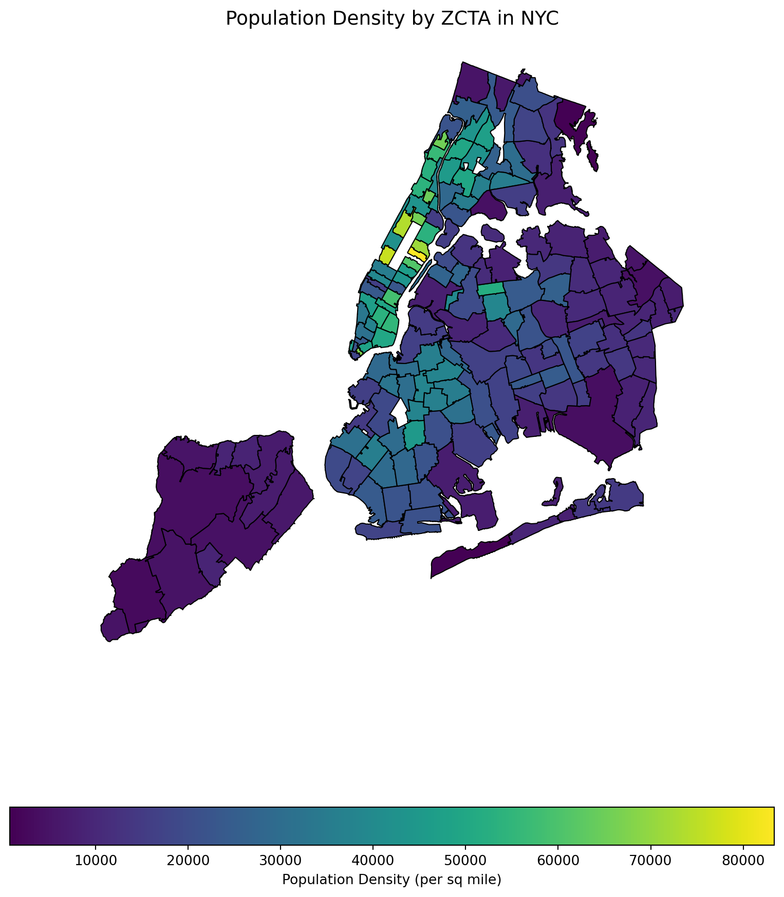
5.5 Cross-platform Data Format Arrow
The CSV format (and related formats like TSV - tab-separated values) for data tables is ubiquitous, convenient, and can be read or written by many different data analysis environments, including spreadsheets. An advantage of the textual representation of the data in a CSV file is that the entire data table, or portions of it, can be previewed in a text editor. However, the textual representation can be ambiguous and inconsistent. The format of a particular column: Boolean, integer, floating-point, text, factor, etc. must be inferred from text representation, often at the expense of reading the entire file before these inferences can be made. Experienced data scientists are aware that a substantial part of an analysis or report generation is often the “data cleaning” involved in preparing the data for analysis. This can be an open-ended task — it required numerous trial-and-error iterations to create the list of different missing data representations we use for the sample CSV file and even now we are not sure we have them all.
To read and export data efficiently, leveraging the Apache Arrow library can significantly improve performance and storage efficiency, especially with large datasets. The IPC (Inter-Process Communication) file format in the context of Apache Arrow is a key component for efficiently sharing data between different processes, potentially written in different programming languages. Arrow’s IPC mechanism is designed around two main file formats:
- Stream Format: For sending an arbitrary length sequence of Arrow record batches (tables). The stream format is useful for real-time data exchange where the size of the data is not known upfront and can grow indefinitely.
- File (or Feather) Format: Optimized for storage and memory-mapped access, allowing for fast random access to different sections of the data. This format is ideal for scenarios where the entire dataset is available upfront and can be stored in a file system for repeated reads and writes.
Apache Arrow provides a columnar memory format for flat and hierarchical data, optimized for efficient data analytics. It can be used in Python through the pyarrow package. Here’s how you can use Arrow to read, manipulate, and export data, including a demonstration of storage savings.
First, ensure you have pyarrow installed on your computer (and preferrably, in your current virtual environment):
pip install pyarrowFeather is a fast, lightweight, and easy-to-use binary file format for storing data frames, optimized for speed and efficiency, particularly for IPC and data sharing between Python and R or Julia.
The following code processes the cleaned data in CSV format from Mohammad Mundiwala and write out in Arrow format.
import pandas as pd

# Read CSV, ensuring 'zip_code' is string and 'crash_datetime' is parsed as datetime
df = pd.read_csv('data/nyc_crashes_cleaned_mm.csv',
                 dtype={'zip_code': str},
                 parse_dates=['crash_datetime'])

# Drop the 'date' and 'time' columns
df = df.drop(columns=['crash_date', 'crash_time'])

# Move 'crash_datetime' to the first column
df = df[['crash_datetime'] + df.drop(columns=['crash_datetime']).columns.tolist()]

df['zip_code'] = df['zip_code'].astype(str).str.rstrip('.0')

df = df.sort_values(by='crash_datetime')

df.to_feather('nyccrashes_cleaned.feather')
Let’s compare the file sizes of the feather format and the CSV format.
import os

# File paths
csv_file = 'data/nyccrashes_2024w0630_by20250212.csv'
feather_file = 'data/nyccrashes_cleaned.feather'

# Get file sizes in bytes
csv_size = os.path.getsize(csv_file)
feather_size = os.path.getsize(feather_file)

# Convert bytes to a more readable format (e.g., MB)
csv_size_mb = csv_size / (1024 * 1024)
feather_size_mb = feather_size / (1024 * 1024)

# Print the file sizes
print(f"CSV file size: {csv_size_mb:.2f} MB")
print(f"Feather file size: {feather_size_mb:.2f} MB")
CSV file size: 0.34 MB
Feather file size: 0.19 MBRead the feather file back in:
#| eval: false
dff = pd.read_feather("data/nyccrashes_cleaned.feather")
dff.shape
5.6 Database with SQL
This section was prepared by Alyssa Horn, a junior Applied Data Analysis major with a domain in Public Policy/Management.
This section explores database operations using SQL in Python, focusing on the contributing_factor_vehicle_1 column of the NYC crash dataset. We’ll use Python’s sqlite3 and pandas libraries for database interaction.
5.6.1 What is a Database?
A collection of related data.
Organized in a way that allows computers to efficiently store, retrieve, and manipulate information.
“Filing system” for large amounts of data that can be easily accessed and analyzed
5.6.1.1 Non-relational Databases
- Ideal for handling large volumes of unstructured or semi-structured data.
- Does not store data in a traditional tabular format with rows and columns like a relational database.
- Allows for more flexible data structures like documents, key-value pairs, graphs, or columns.
5.6.1.2 Relational Databases
- Stores data in tables with rows (records) and columns (attributes).
- Each table has a primary key to uniquely identify records.
- Allows you to easily access and understand how different pieces of data are connected to each other.
- Example: In a phone book, each contact has a unique ID, name, phone number, and address.
5.6.2 What is SQL?
- Structured Query Language for managing and querying relational databases.
- Helps you store, retrieve, update, and delete data easily using simple commands in Python.
- Using sqlite3, you can run SQL queries directly from your Python code to interact with your database seamlessly.
5.6.2.1 CRUD Model
The four most basic operations that can be performed with most traditional database systems and they are the backbone for interacting with any database.
- Create: Insert new records.
- Read: Retrieve data.
- Update: Modify existing records.
- Delete: Remove records.
5.6.2.2 What can SQL do?
- Execute queries against a database
- Retrieve data from a database
- Insert records in a database
- Update records in a database
- Delete records from a database
- Create new databases
- Create new tables in a database
- Create stored procedures in a database
- Create views in a database
- Set permissions on tables, procedures, and views
5.6.2.3 Key Statements
- Create a cursor object to interact with the database
cursor.executeexecutes a single SQL statementconn.commitsaves all changes madequery =requests specific information from database
5.6.3 Setting up the Database
5.6.3.1 Read in the datatset and store dataframe as SQL table
We start by importing necessary packages and reading in the cleaned nyccrashes feather.
- Use
data.to_sqlto store dataframe as an SQL table.
import sqlite3
import pandas as pd

# Create a database and load the NYC crash data
db_path = 'nyc_crash.db'
conn = sqlite3.connect(db_path)
#The conn object acts as a bridge between Python and the database,
#allowing you to execute SQL queries and manage data.

# Load Feather
data = pd.read_feather("data/nyccrashes_cleaned.feather")

# create crash_date and crash_time columns
data["crash_date"] = pd.to_datetime(data["crash_datetime"]).dt.date
data["crash_time"] = pd.to_datetime(data["crash_datetime"]).dt.strftime("%H:%M:%S")

# Drop the original datetime column (optional)
data.drop(columns=["crash_datetime"], inplace=True)

# Store DataFrame as a SQL table
data.to_sql('nyc_crashes', conn, if_exists='replace', index=False)18755.6.3.2 Display the Table
We can display the table by querying all (or some) of the data and using the .head() command
# Query to select all data (or limit rows to avoid overload)
query = "SELECT * FROM nyc_crashes LIMIT 10;"

# Load the data into a pandas DataFrame
nyc_crashes_data = pd.read_sql_query(query, conn)

# Display the DataFrame
nyc_crashes_data.head(5)| borough | zip_code | latitude | longitude | location | on_street_name | cross_street_name | off_street_name | number_of_persons_injured | number_of_persons_killed | ... | contributing_factor_vehicle_4 | contributing_factor_vehicle_5 | collision_id | vehicle_type_code_1 | vehicle_type_code_2 | vehicle_type_code_3 | vehicle_type_code_4 | vehicle_type_code_5 | crash_date | crash_time | |
|---|---|---|---|---|---|---|---|---|---|---|---|---|---|---|---|---|---|---|---|---|---|
| 0 | None | NaN | NaN | NaN | (0.0, 0.0) | None | None | GOLD STREET | 0 | 0 | ... | None | None | 4736746 | Sedan | Sedan | None | None | None | 2024-06-30 | 17:30:00 |
| 1 | None | NaN | NaN | NaN | None | BELT PARKWAY RAMP | None | None | 0 | 0 | ... | None | None | 4736768 | Station Wagon/Sport Utility Vehicle | Station Wagon/Sport Utility Vehicle | None | None | None | 2024-06-30 | 00:32:00 |
| 2 | BROOKLYN | 11235.0 | 40.58106 | -73.96744 | (40.58106, -73.96744) | None | None | 2797 OCEAN PARKWAY | 0 | 0 | ... | None | None | 4737060 | Station Wagon/Sport Utility Vehicle | None | None | None | None | 2024-06-30 | 07:05:00 |
| 3 | MANHATTAN | 10021.0 | 40.76363 | -73.95330 | (40.76363, -73.9533) | FDR DRIVE | None | None | 0 | 0 | ... | None | None | 4737510 | Sedan | None | None | None | None | 2024-06-30 | 20:47:00 |
| 4 | BROOKLYN | 11222.0 | 40.73046 | -73.95149 | (40.73046, -73.95149) | GREENPOINT AVENUE | MC GUINNESS BOULEVARD | None | 0 | 0 | ... | None | None | 4736759 | Bus | Box Truck | None | None | None | 2024-06-30 | 10:14:00 |
5 rows × 29 columns
5.6.4 Normalizing the Database with a Lookup Table
5.6.4.1 Create the lookup table
Create the lookup table using the create table command with the corresponding column names.
# Connect to the SQLite database
cursor = conn.cursor()

cursor.execute('''
CREATE TABLE IF NOT EXISTS contributing_factor_lookup (
    factor_id INTEGER PRIMARY KEY AUTOINCREMENT,
    factor_description TEXT UNIQUE
)
''')
print("Lookup table created successfully.")
Lookup table created successfully.5.6.4.2 Populate the Lookup Table with Distinct Values
Populate the lookup table with the values contained in contributing_factor_vehicle_1.
cursor.execute('''
INSERT OR IGNORE INTO contributing_factor_lookup (factor_description)
SELECT DISTINCT contributing_factor_vehicle_1
FROM nyc_crashes
WHERE contributing_factor_vehicle_1 IS NOT NULL;
''')
print("Lookup table populated with distinct contributing factors.")
Lookup table populated with distinct contributing factors.5.6.4.3 Update the Original Table to Include factor_id
Use ALTER TABLE to add factor_id column into original table.
cursor.execute('''
ALTER TABLE nyc_crashes ADD COLUMN factor_id INTEGER;
''')
print("Added 'factor_id' column to nyc_crashes table.")
Added 'factor_id' column to nyc_crashes table.5.6.4.4 Update the Original Table with Corresponding Codes
Use UPDATE command to update table with factor descriptions.
cursor.execute('''
UPDATE nyc_crashes
SET factor_id = (
    SELECT factor_id
    FROM contributing_factor_lookup
    WHERE contributing_factor_vehicle_1 = factor_description
)
WHERE contributing_factor_vehicle_1 IS NOT NULL;
''')
print("Updated nyc_crashes with corresponding factor IDs.")
Updated nyc_crashes with corresponding factor IDs.5.6.4.5 Query with a Join to Retrieve Full Descriptions
Use JOIN command to recieve contributing factor descriptions from factor_id.
query = '''
SELECT n.*, l.factor_description
FROM nyc_crashes n
JOIN contributing_factor_lookup l ON n.factor_id = l.factor_id
LIMIT 10;
'''

# Load the data into a pandas DataFrame
result_df = pd.read_sql_query(query, conn)

# Commit changes
conn.commit()

result_df.head()| borough | zip_code | latitude | longitude | location | on_street_name | cross_street_name | off_street_name | number_of_persons_injured | number_of_persons_killed | ... | collision_id | vehicle_type_code_1 | vehicle_type_code_2 | vehicle_type_code_3 | vehicle_type_code_4 | vehicle_type_code_5 | crash_date | crash_time | factor_id | factor_description | |
|---|---|---|---|---|---|---|---|---|---|---|---|---|---|---|---|---|---|---|---|---|---|
| 0 | None | NaN | NaN | NaN | (0.0, 0.0) | None | None | GOLD STREET | 0 | 0 | ... | 4736746 | Sedan | Sedan | None | None | None | 2024-06-30 | 17:30:00 | 1 | Passing Too Closely |
| 1 | None | NaN | NaN | NaN | None | BELT PARKWAY RAMP | None | None | 0 | 0 | ... | 4736768 | Station Wagon/Sport Utility Vehicle | Station Wagon/Sport Utility Vehicle | None | None | None | 2024-06-30 | 00:32:00 | 2 | Unspecified |
| 2 | BROOKLYN | 11235.0 | 40.58106 | -73.96744 | (40.58106, -73.96744) | None | None | 2797 OCEAN PARKWAY | 0 | 0 | ... | 4737060 | Station Wagon/Sport Utility Vehicle | None | None | None | None | 2024-06-30 | 07:05:00 | 2 | Unspecified |
| 3 | MANHATTAN | 10021.0 | 40.76363 | -73.95330 | (40.76363, -73.9533) | FDR DRIVE | None | None | 0 | 0 | ... | 4737510 | Sedan | None | None | None | None | 2024-06-30 | 20:47:00 | 2 | Unspecified |
| 4 | BROOKLYN | 11222.0 | 40.73046 | -73.95149 | (40.73046, -73.95149) | GREENPOINT AVENUE | MC GUINNESS BOULEVARD | None | 0 | 0 | ... | 4736759 | Bus | Box Truck | None | None | None | 2024-06-30 | 10:14:00 | 1 | Passing Too Closely |
5 rows × 31 columns
5.6.4.6 Display Table With factor.id
Since we added factor_id column to dataframe, we can now display the table including the factor_id column using a query.
# Query to select all data (or limit rows to avoid overload)
query = "SELECT * FROM nyc_crashes LIMIT 10;"

# Load the data into a pandas DataFrame
nyc_crashes_data = pd.read_sql_query(query, conn)

# Display the DataFrame
nyc_crashes_data.head()| borough | zip_code | latitude | longitude | location | on_street_name | cross_street_name | off_street_name | number_of_persons_injured | number_of_persons_killed | ... | contributing_factor_vehicle_5 | collision_id | vehicle_type_code_1 | vehicle_type_code_2 | vehicle_type_code_3 | vehicle_type_code_4 | vehicle_type_code_5 | crash_date | crash_time | factor_id | |
|---|---|---|---|---|---|---|---|---|---|---|---|---|---|---|---|---|---|---|---|---|---|
| 0 | None | NaN | NaN | NaN | (0.0, 0.0) | None | None | GOLD STREET | 0 | 0 | ... | None | 4736746 | Sedan | Sedan | None | None | None | 2024-06-30 | 17:30:00 | 1 |
| 1 | None | NaN | NaN | NaN | None | BELT PARKWAY RAMP | None | None | 0 | 0 | ... | None | 4736768 | Station Wagon/Sport Utility Vehicle | Station Wagon/Sport Utility Vehicle | None | None | None | 2024-06-30 | 00:32:00 | 2 |
| 2 | BROOKLYN | 11235.0 | 40.58106 | -73.96744 | (40.58106, -73.96744) | None | None | 2797 OCEAN PARKWAY | 0 | 0 | ... | None | 4737060 | Station Wagon/Sport Utility Vehicle | None | None | None | None | 2024-06-30 | 07:05:00 | 2 |
| 3 | MANHATTAN | 10021.0 | 40.76363 | -73.95330 | (40.76363, -73.9533) | FDR DRIVE | None | None | 0 | 0 | ... | None | 4737510 | Sedan | None | None | None | None | 2024-06-30 | 20:47:00 | 2 |
| 4 | BROOKLYN | 11222.0 | 40.73046 | -73.95149 | (40.73046, -73.95149) | GREENPOINT AVENUE | MC GUINNESS BOULEVARD | None | 0 | 0 | ... | None | 4736759 | Bus | Box Truck | None | None | None | 2024-06-30 | 10:14:00 | 1 |
5 rows × 30 columns
5.6.5 Inserting Data
New records (rows) can be added into a database table. The INSERT INTO statement is used to accomplish this task. When you insert data, you provide values for one or more columns in the table.
INSERT INTO table_name (columns) VALUES (values
Insert a new crash record into the nyc_crashes table with the date 06/30/2024, time 10:15, location BROOKLYN, and contributing factor “Driver Inattention/Distraction”.
cursor = conn.cursor()

# Adds a crash on 06/30/2024 at 10:15 in
# Brooklyn due to Inattention/Distraction
cursor.execute("""
INSERT INTO nyc_crashes (crash_date, crash_time,
borough, contributing_factor_vehicle_1)
VALUES ('2024-06-30', '10:15:00', 'BROOKLYN',
'Driver Inattention/Distraction')
""")

conn.commit()
5.6.5.1 Verify the record exists
We can use a query for a specific data point to verify if addition was successful.
query_before = """
SELECT * FROM nyc_crashes
WHERE crash_date = '2024-06-30'
AND crash_time = '10:15:00'
AND borough = 'BROOKLYN';
"""

before_deletion = pd.read_sql_query(query_before, conn)
print("Before Deletion:")
before_deletion
Before Deletion:| borough | zip_code | latitude | longitude | location | on_street_name | cross_street_name | off_street_name | number_of_persons_injured | number_of_persons_killed | ... | contributing_factor_vehicle_5 | collision_id | vehicle_type_code_1 | vehicle_type_code_2 | vehicle_type_code_3 | vehicle_type_code_4 | vehicle_type_code_5 | crash_date | crash_time | factor_id | |
|---|---|---|---|---|---|---|---|---|---|---|---|---|---|---|---|---|---|---|---|---|---|
| 0 | BROOKLYN | None | None | None | None | None | None | None | None | None | ... | None | None | None | None | None | None | None | 2024-06-30 | 10:15:00 | None |
1 rows × 30 columns
5.6.6 Deleting Data
Use DELETE FROM statement to delete data
delete_query = """
DELETE FROM nyc_crashes
WHERE crash_date = '2024-06-30'
AND crash_time = '10:15:00'
AND borough = 'BROOKLYN'
AND contributing_factor_vehicle_1 = 'Driver Inattention/Distraction';
"""

cursor.execute(delete_query)
conn.commit()
5.6.6.1 Verify the deletion
We can use a query for a specific data point to verify if deletion was successful.
query_after = """
SELECT * FROM nyc_crashes
WHERE crash_date = '2024-06-30'
AND crash_time = '10:15:00'
AND borough = 'BROOKLYN';
"""

after_deletion = pd.read_sql_query(query_after, conn)
print("After Deletion:")
after_deletion
After Deletion:| borough | zip_code | latitude | longitude | location | on_street_name | cross_street_name | off_street_name | number_of_persons_injured | number_of_persons_killed | ... | contributing_factor_vehicle_5 | collision_id | vehicle_type_code_1 | vehicle_type_code_2 | vehicle_type_code_3 | vehicle_type_code_4 | vehicle_type_code_5 | crash_date | crash_time | factor_id |
|---|
0 rows × 30 columns
5.6.7 Querying the data
Querying the data means requesting specific information from a database. In SQL, queries are written as commands to retrieve, filter, group, or sort data based on certain conditions. The goal of querying is to extract meaningful insights or specific subsets of data from a larger dataset.
SELECT DISTINCTretrieves unique values from a columnpd.read_sql_query()executes the SQL query and returns the result as a DataFrame —
5.6.7.1 Query to find distinct contributing factors
This query selects the distinct contributing factors from the contributing_factor_vehicle_1 column.
query = "SELECT DISTINCT contributing_factor_vehicle_1 FROM nyc_crashes;"

factors = pd.read_sql_query(query, conn)

factors.head(5)| contributing_factor_vehicle_1 | |
|---|---|
| 0 | Passing Too Closely |
| 1 | Unspecified |
| 2 | Driver Inattention/Distraction |
| 3 | Failure to Yield Right-of-Way |
| 4 | Other Vehicular |
5.6.7.2 Can query using factor.id
This query selects the distinct contributing factors using the factor_id column.
query = """
SELECT DISTINCT n.factor_id, l.factor_description
FROM nyc_crashes n
JOIN contributing_factor_lookup l ON n.factor_id = l.factor_id
WHERE n.factor_id IS NOT NULL;
"""

factors = pd.read_sql_query(query, conn)
factors.head(5)| factor_id | factor_description | |
|---|---|---|
| 0 | 1 | Passing Too Closely |
| 1 | 2 | Unspecified |
| 2 | 3 | Driver Inattention/Distraction |
| 3 | 4 | Failure to Yield Right-of-Way |
| 4 | 5 | Other Vehicular |
5.6.8 Analyzing contributing_factor_vehicle_1
SELECTChoose columns to retrieveCOUNTCount rows for each groupGROUP BYGroup rows that have the same values in specific columnsORDER BYSort results by the count in descending order
5.6.8.1 Insights into contributing_factor_vehicle_1
- Identify the most common contributing factors.
- Understand trends related to vehicle crash causes.
factor_count = pd.read_sql_query("""
SELECT contributing_factor_vehicle_1, COUNT(*) AS count
FROM nyc_crashes
GROUP BY contributing_factor_vehicle_1
ORDER BY count DESC;
""", conn)

factor_count.head(10)| contributing_factor_vehicle_1 | count | |
|---|---|---|
| 0 | Unspecified | 473 |
| 1 | Driver Inattention/Distraction | 447 |
| 2 | Failure to Yield Right-of-Way | 116 |
| 3 | Following Too Closely | 104 |
| 4 | Unsafe Speed | 82 |
| 5 | Passing or Lane Usage Improper | 74 |
| 6 | Traffic Control Disregarded | 66 |
| 7 | Other Vehicular | 63 |
| 8 | Passing Too Closely | 57 |
| 9 | Alcohol Involvement | 57 |
5.6.9 Visualizing Analysis
Can use Plotnine to visualize our Analysis for contributing_factor_vehicle_1 in a chart.
from plotnine import ggplot, aes, geom_bar, theme_minimal, coord_flip, labs

db_path = 'nyc_crash.db'
conn = sqlite3.connect(db_path)

# Query to get the contributing factor counts
factor_count = pd.read_sql_query("""
SELECT contributing_factor_vehicle_1, COUNT(*) AS count
FROM nyc_crashes
GROUP BY contributing_factor_vehicle_1
ORDER BY count DESC;
""", conn)

# Create a bar chart using plotnine
chart = (
    ggplot(factor_count, aes(x='reorder(contributing_factor_vehicle_1, count)'
                             , y='count')) +
    geom_bar(stat='identity', fill='steelblue') +
    coord_flip() +  # Flip for better readability
    theme_minimal() +
    labs(title='Top Contributing Factors to NYC Crashes',
         x='Contributing Factor',
         y='Number of Incidents')
)

chart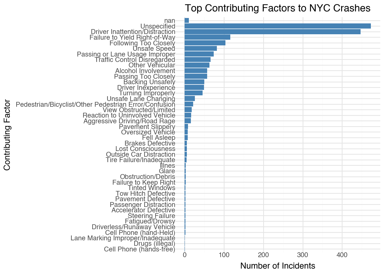
5.6.10 Conclusion
- SQL in Python is powerful for handling structured data.
- sqlite3 and pandas simplify database interactions.
- Analyzing crash data helps understand key contributing factors for traffic incidents. —
5.6.11 Further Readings:
5.8 Imputation Methods for Missing Data
This section was prepared by Sebastian Symula, a Junior Statistical Data Science major with a domain in statistics and a minor in math graduating in the fall.
This section will serve as an introduction into what data imputation is, when to do it, as well as comparing and contrasting a few different methods of imputation.
5.8.1 What is Data Imputation?
In practice, most datasets will have missing values. This can be due to things like faulty equipment, nonresponse, or the data not existing in the first place.
When data is missing, you have two options:
- Ignore it (Complete Case Analysis): We only use complete rows without missing data for our analysis.
- Impute it: We fill in missing values using some statistical method.
Types of Missing Data:
Missing Completely at Random (MCAR):This is the best case scenario. There is no pattern to be observed with missing and observed data. The full rows can be treated as an independent subset of the full dataset. This does not introduce bias and is usually not a realistic assumption. Each row has same chance of being missing.
Missing at Random (MAR): Missing data can be explained by observed data. missingness of data is related to observed variables, but not to the missing values themselves. Therefore, the mechanism of missingness can be modeled with observed data.
Missing Not at Random (MNAR): This is when the missingness may say something about the true value, due to some unobserved data. So the fact that the value is missing has an impact on the true value. Do NOT impute in this case.
Types of Missing Data Example:
Let’s imagine we have a dataset where one column is gender and the other is the respondent’s happiness score from a survey.
- MCAR: If we see a relatively even spread of missing values between men and women. In this case the complete cases would be an independent subset of the dataset and we could run complete case analysis without any bias provided the missing data isn’t a large portion of our set.
- MAR: If we see a pattern of more missing values for men, but we assume this is due to men not finishing the survey and does not correlate with their happiness score. In this case we can use the observed cases for men to impute the missing ones.
- MNAR: If we think someone who’s less happy might be less likely to complete the survey. Can’t use observed values to predict missing ones.
5.8.2 Inspecting Missingness
Let’s create a complete dataset, then introduce MAR data:
import pandas as pd
import numpy as np

np.random.seed(10)
data = {
    'ID': np.arange(1, 3000 + 1),
    'Age': np.random.randint(18, 60,3000),
    'Salary': np.random.randint(30000, 100000, 3000),
    'Department': np.random.choice(['Sales', 'HR', 'IT', 'Finance'], 3000),
    'Location': np.random.choice(['Remote', 'Hybrid'], 3000),
    'Tenure': np.random.randint(0,35, 3000)
}
df = pd.DataFrame(data)
Dataset has 6 columns and 3000 rows.
Introducing Missing Values:
sal_prob = np.clip((df['Age'] - 30) / 40, 0, 1)
sal_mask = np.random.uniform(0, 1, size=3000) < sal_prob
dep_prob = np.clip((35 - df['Tenure']) / 35, 0, 1)
dep_mask = np.random.uniform(0, 1, size=3000) < dep_prob
ten_prob = np.where(df['Location'] == 'Hybrid', 0.6, 0.1)
ten_mask = np.random.uniform(0, 1, size=3000) < ten_prob
# Create dataset with missing values
df_missing = df.copy()
df_missing.loc[sal_mask, 'Salary'] = np.nan
df_missing.loc[dep_mask, 'Department'] = np.nan
df_missing.loc[ten_mask, 'Tenure'] = np.nan
missing_vals = df_missing.isnull()
Probability of Salary being missing increases as Age increases
Probability of Department being missing increases as Tenure decreases
Probability of Tenure being missing is greater if Location is Hybrid
df_missing.isna().sum()ID 0
Age 0
Salary 785
Department 1573
Location 0
Tenure 1052
dtype: int64isna().sum() is a good place to start when looking at missing data. It provides the sum of missing data by column.
Inspecting Missingness: Age vs Salary
import seaborn as sns
import matplotlib.pyplot as plt
plt.figure(figsize=(10, 6))
sns.scatterplot(data=df_missing, x='Age', y='Salary', alpha=0.6, color='blue')
plt.title("MAR Missing Pattern: Income Missing More for Older Individuals")
plt.show()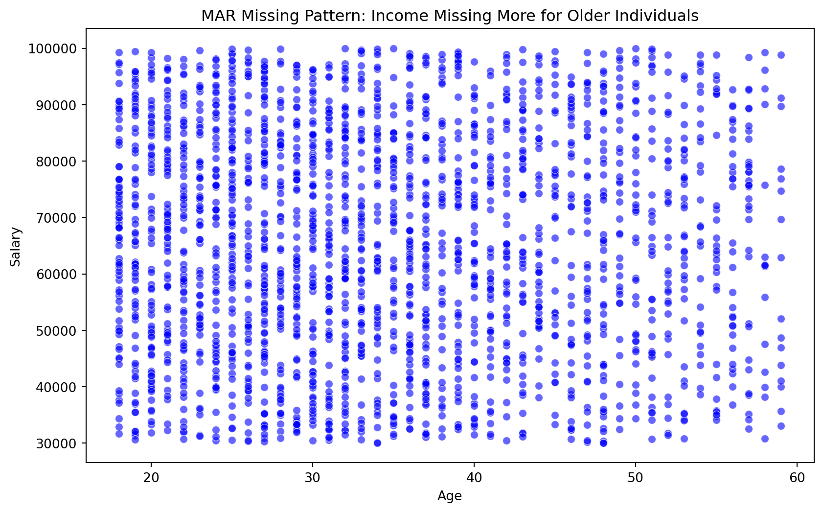
We can see that there is a trend of more missing values for Salary as Age increases.
Inspecting Missingness: Tenure vs Department
df_missing['dep_missing'] = df_missing['Department'].isnull().astype(int)

# Bin Tenure for easier visualization
df_missing['tenure_binned'] = pd.cut(df['Tenure'], bins=[0, 5, 10, 20, 30, 35],
                             labels=['0-5', '6-10', '11-20', '21-30', '30+'],
                             include_lowest=True)
# Bar plot to show % of missingness per tenure bin
plt.figure(figsize=(8, 5))
sns.barplot(x=df_missing['tenure_binned'], y=df_missing['dep_missing'], estimator=np.mean, palette="coolwarm")
plt.xlabel("Tenure (Binned)")
plt.ylabel("Proportion of Department Missing")
plt.title("Proportion of Missing Department Values by Tenure")
plt.show()
df_missing.drop(columns=['dep_missing','tenure_binned'],inplace= True)
/var/folders/cq/5ysgnwfn7c3g0h46xyzvpj800000gn/T/ipykernel_14254/955409734.py:9: FutureWarning:
Passing `palette` without assigning `hue` is deprecated and will be removed in v0.14.0. Assign the `x` variable to `hue` and set `legend=False` for the same effect.
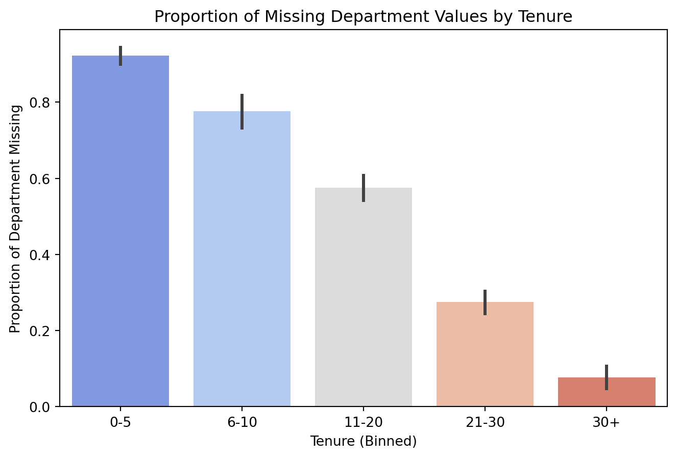
There are more missing values for Department as Tenure decreases.
Inspecting Missingness: Location vs Tenure
plt.figure(figsize=(8, 5))
df_missing['missingflag_ten'] = df_missing['Tenure'].isnull()
from sklearn.impute import MissingIndicator
indicator = MissingIndicator(missing_values=np.nan, features='all')
mask_all = indicator.fit_transform(df_missing)
# Plot scatter with missingness indicated by color
plt.figure(figsize=(8, 5))
sns.countplot(data=df_missing, x='Location', hue=df_missing['missingflag_ten'], palette={True: 'red', False: 'blue'})
df_missing.drop(columns = ['missingflag_ten'], inplace = True)
# Customize the plot
plt.legend()
plt.title("Missing Tenure by Location: Hybrid vs Remote")
plt.xlabel("Location")
plt.ylabel("Count")
plt.show()
<Figure size 768x480 with 0 Axes>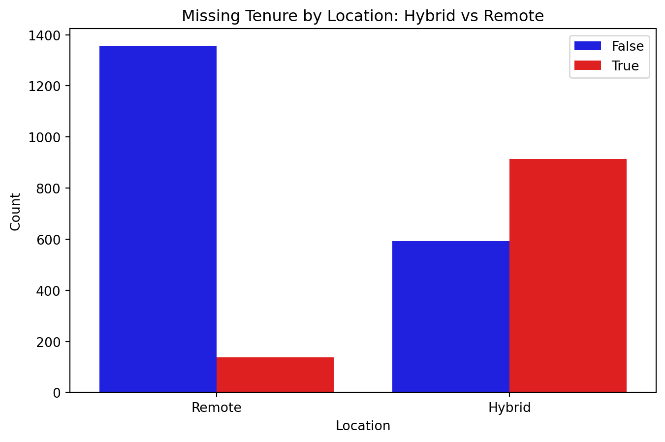
More missing values for Tenure when Location is Hybrid.
When Is Imputing a Good Idea?
Imputing might be the right decision if:
It makes sense in the context of the data. Sometimes missing values are expected.
It wouldn’t introduce extra bias. Depends on the kind of missing data.
Deleting would result in losing important data.
The computational cost isn’t too great.
The missing data is greater than 5 percent of the dataset.
5.8.3 Methods of Imputation
5.8.3.1 Simple Methods
Mean
Median
Mode
These can be a good initial option but will underestimate error.
Fast and easy computationally.
Will mess up visuals. There will be large clumps around the mean/median/mode.
Mean/Mode Imputation
For simplicity, we will exclusively be using functions from sklearn throughout. Specifically sklearn.impute.
# importing and initialize imputations
from sklearn.impute import SimpleImputer
imp_mean = SimpleImputer(missing_values=np.nan, strategy='mean')
imp_mode = SimpleImputer(missing_values=np.nan, strategy='most_frequent')

## making a copy dataframe with missing values for imputation use
mean_df = df_missing.copy()

# imputing numeric and categorical features separately
mean_df[['Salary', 'Tenure']] = imp_mean.fit_transform(mean_df[['Salary', 'Tenure']])
mean_df[['Department']] = imp_mode.fit_transform(mean_df[['Department']])
Realistically, we don’t need to use these functions. We could manually impute the mean or mode.
Evaluating Mean/Mode Imputation:
# calculating rmse
from sklearn.metrics import mean_squared_error
rmse_salary_simple = np.sqrt(mean_squared_error(df['Salary'], mean_df['Salary']))
rmse_tenure_simple = np.sqrt(mean_squared_error(df['Tenure'], mean_df['Tenure']))

# calculating accuracy
correct_imputations = (df[missing_vals]['Department'] == mean_df[missing_vals]['Department']).sum()
total_imputed = missing_vals['Department'].sum()
categorical_accuracy = correct_imputations / total_imputed

print(f'Tenure Error: {rmse_tenure_simple} years')
print(f'Salary Error: ${rmse_salary_simple}')
print(f'Department Accuracy: {categorical_accuracy}')
Tenure Error: 6.0706196465053335 years
Salary Error: $10658.00027447137
Department Accuracy: 0.24284806102987921For evaluating accuracy of imputations, we will be using mean squared error for continuous variables and proportion of correct imputations for categorical data.
KNN Imputation
One of the most popular methods of imputation. Finds \(k\) nearest neighbors that don’t have missing values for the given column. Uses the mean of these values to impute missing value.
- Uses Euclidean distance to find nearest neighbors
- Becomes computationally expensive for higher values of \(k\)
- Can be used for MCAR and MAR
KNN Imputation Example:
# importing and initializing imputer
from sklearn.impute import KNNImputer
from sklearn.preprocessing import OrdinalEncoder
knn_df = df_missing.copy()

# encoding the categorical column (doesn't work on strings)
encoder = OrdinalEncoder(handle_unknown='use_encoded_value', unknown_value=np.nan)
knn_df[['Department','Location']] = encoder.fit_transform(knn_df[['Department','Location']])

# imputing the dataFrame using k = 8
imputer = KNNImputer(n_neighbors=8, weights="uniform")
knn_df_imputed = imputer.fit_transform(knn_df)
# converting back to DataFrame
knn_df = pd.DataFrame(knn_df_imputed, columns=knn_df.columns)
# rounding the encoded column to integers (sometimes knn doesn't return # ints)
knn_df['Department'] = np.round(knn_df['Department']).astype(int)

# reverse encoding back to strings for accuracy evaluation
knn_df[['Department','Location']] = encoder.inverse_transform(knn_df[['Department','Location']])- This KNN Imputer only works with numeric data, so we encoded the categorical features.
- The number of neighbors, \(k\) can be tuned. In this case we choose \(k\) = 8. Typically 5-10 is a good number.
KNN Accuracy:
# finding rmse for Salary and Tenure
rmse_salary_knn = np.sqrt(mean_squared_error(df['Salary'], knn_df['Salary']))
rmse_tenure_knn = np.sqrt(mean_squared_error(df['Tenure'], knn_df['Tenure']))

correct_imputations = (df[missing_vals]['Department'] == knn_df[missing_vals]['Department']).sum()
total_imputed = missing_vals['Department'].sum()
categorical_accuracy = correct_imputations / total_imputed

print(f'Tenure Error: {rmse_tenure_knn} years')
print(f'Salary Error: ${rmse_salary_knn}')
print(f'Department Accuracy: {categorical_accuracy}')
Tenure Error: 6.227130659461065 years
Salary Error: $11301.554318226681
Department Accuracy: 0.26573426573426573- The root MSE for both Tenure and Salary increased
- Department accuracy increased slightly over the 1 in 4 random guessing that was used with mode imputation.
Problems with Single Imputation
All these examples have been methods of single imputation, in which one value is imputed for each missing value.
Only having one value is understating the uncertainty of the true value and when we use single imputation, the imputed value will almost always be incorrect.
Since we’re very uncertain about the true values, we should impute multiple times to correctly account for uncertainty.
5.8.3.2 Multiple Imputation
Execute another imputation technique (like KNN) \(m\) times on randomly sampled subsets that don’t have missing values for the given column. This creates a set of possible values instead of just one. We then perform statistical analysis on each of the \(m\) complete datasets and pool the results of the analysis.
- Can become computationally expensive for large datasets or large values of \(m\).
- \(m\) can take on any value. Common range is 20-100, but generally bigger is better.
Multiple Imputation by Chained Equations (MICE)
- Step 1: A simple imputation, such as imputing the mean, is performed for every missing value in the dataset. These mean imputations can be thought of as “place holders.”
- Step 2: The “place holder” mean imputations for one variable (“var”) are set back to missing.
- Step 3: The observed values from the variable “var” in Step 2 are regressed on the other variables in the imputation model.
- Step 4: This process is repeated for each feature with missing values, then the entire process is repeated for a given number of iterations until the algorithm reaches convergence (imputed values yield similar results after each iteration).
- This forms 1 imputed dataset. We repeat this process \(m\) times.
Using statsmodels.imputation.mice
- We will be using the
MICEDatafunction fromstatsmodels.imputation. micefor multiple imputation. k_pmm: This is the size of the sample used to perform predictive mean matching. Predictive mean matching is similar to KNN in that it uses similar rows to impute.perturbation_method: Adds random noise to imputations to account for uncertainty. We use ‘gaussian’ for this because we are adding noise generated from a normal distribution.
MI Example
from statsmodels.imputation.mice import MICEData
import statsmodels.api as sm
import numpy as np
from sklearn.preprocessing import OrdinalEncoder

# copying data and encode categorical variables
df_mi = df_missing.copy()
encoder = OrdinalEncoder(handle_unknown='use_encoded_value', unknown_value=np.nan)
df_mi[['Department', 'Location']] = encoder.fit_transform(df_mi[['Department', 'Location']]).astype(int)

# performing Multiple Imputation
mice_data = MICEData(df_mi,k_pmm = 30, perturbation_method='gaussian')
m = 20  # Number of imputed datasets
imputed_datasets = []
for _ in range(m):
    mice_data.update_all()  # Perform one imputation step
    imputed_datasets.append(mice_data.data.copy())  # Store a copy of the imputed dataset
/var/folders/cq/5ysgnwfn7c3g0h46xyzvpj800000gn/T/ipykernel_14254/3889701920.py:9: RuntimeWarning: invalid value encountered in castPooling MI Results
we have multiple regression models formed from multiple imputed datasets, but we need one final model.
To achieve this, we pool the results using Rubin’s combination rules.
For parameter estimates, we simply take the average.
For within imputation variance, we take the average of variances.
For between imputation variance, we use the equation given by:
\(b = \frac{1}{m - 1} \sum_{i = 1}^{m} (\theta_i - \hat{\theta})^2\).
- For pooled total variance of imputed datasets, we use the equation:
\(t = w + (1 + 1/m)*b\),
where \(w\) is the within imputation variance, \(b\) is the between imputation variance, \(m\) is the total number of imputed datasets, \(\theta\) is a parameter estimate, and \(\hat{theta}\) is our pooled parameter estimate.
MI Results
Here we fit a linear regression model to each of the 20 imputed dataframes.
# fitting regression models on imputed datasets one at a time
results = [sm.OLS(df['Salary'], sm.add_constant(df[['Department', 'Location','Tenure']])).fit() for df in imputed_datasets]
# pooling estimates using Rubin's Rules (shown above)
params = np.array([res.params for res in results])
bse = np.array([res.bse for res in results])

pooled_means = params.mean(axis=0)
pooled_se = np.sqrt(bse.mean(axis=0) + ((1 + 1/m) * params.var(axis=0, ddof=1)))
print("Pooled Coefficients:\n", pooled_means)
print("\nPooled Standard Errors:\n", pooled_se)
Pooled Coefficients:
[ 1.47442228e-33 -7.13048516e-15 7.34262297e-34 2.44380349e-32]
Pooled Standard Errors:
[5.27258975e-18 1.15950487e-08 3.72081993e-18 2.14656952e-17]The first coefficient/se is for the intercept.
5.8.4 Conclusions
- Not everything needs to be imputed, we need to consider the context of the data. If we suspect that the missing data is MNAR, we do not impute.
- Need to weigh computational cost with accuracy. Multiple imputation can be difficult on large datasets.
- Overall, multiple imputation is a safe bet.
Imputing in R:
These examples were all done in python, because that is the language we’ve used for this class. However, R has much more sophisticated packages and functions for imputing. Specifically the mice package in R has plenty of options for multiple imputation, with a lot of documentation available.
I would recommend checking this out!
5.8.5 Further Readings
5.9 Using NetCDF data
This section was contributed by Noah Kravette. I am a Ph.D. student in Climate Modeling at the University of Connecticut. My research focuses on radiative forcing, climate feedbacks, and climate sensitivities. I use NetCDF data because of how often climate scientists store, visualize, and manipulate climate data using the NetCDF data frame.
5.9.1 What is NetCDF?
NetCDF stands for Network Common Data Format. It is an array-based data format used widely across climate science, oceanography, meteorology, and atmospheric modeling. NetCDF was created by the Unidata Program Center at UCAR in the 1980s and provides a standard way to store, organize, and share scientific data across disciplines.
NetCDF files are particularly useful for multidimensional datasets. Which are datasets that have many dimensions such as time. For example:
Temperature(time, altitude, latitude, longitude).NetCDF files have both the official data and metadata. This makes them self-describing and easily portable across platforms and programming languages.
5.9.2 History of NetCDF
Before NetCDF, researchers used many incompatible formats. These datasets were often not reused outside of individual labs or groups. So Glen Davis developed the first version of NetCDF in 1988, from NASA’s Common Data Format (CDF). From then, NetCDF has become the standard for Earth system model outputs and observational datasets.
5.9.3 Key Features of NetCDF
- Self-describing: Metadata and data are stored together.
- Portable: Works on many operating systems or languages.
- Appendable: New data can be added without overwriting old data.
- Scalable: Supports multidimensional arrays with fast access.
- Sharable: Multiple readers, one writer.
- Archivable: Maintains backward compatibility.
5.9.4 NetCDF Data Model and Structure
The NetCDF data model includes:
- Dimensions: The shape of data (e.g., time, lat, lon).
- Variables: Has the actual data (e.g., temperature).
- Attributes: The metadata describing the variables.
- Data types: Storage precision for data (e.g., float32).
5.9.5 Languages and Libraries
NetCDF is supported in many languages:
- Official APIs: C, C++, Fortran, Java
- Community-supported: Python, R, MATLAB, Julia, Ruby
In Python, the most common libraries for working with NetCDF:
xarray: High-level, labeled multidimensional arrays.netCDF4: Low-level NetCDF interface.matplotlib,cartopy: For plotting geospatial data.
5.9.6 Common Tools for NetCDF
There are many different ways to use and manipulate NetCDF. Below are some common examples and tips.
5.9.6.1 Command-line tools:
ncdump: shows metadata.ncgen: creates NetCDF files from CDL text.ncview: basic GUI viewer for spatial checks (requires XQuartz).
5.9.6.2 NCO tools:
ncks: extract, append, or subset data Example:ncks -A -v variable name.TS.nc new_output.ncncrename: rename variables or dimensionsncrename -O -v TS,ts name.TS.nc name.ts.ncncap2: modify or create new variablesncap2 -O -s 'ts=double(ts)' name.ts.nc name.ts.ncncrcat: concatenate files along a record dimension
5.9.7 Using ncview with XQuartz
To visualize NetCDF data quickly, use ncview. This opens a basic interface that can scroll through time steps or other dimensions for your variables. However it requires XQuartz to be installed onto your operating system.
ncview netcdf_file.ncAs long as you have XQuartz installed and working, ncview will pop up and then you can use it to see your data easily before any coding diagnostic step.
5.9.8 Python Example: TOA Net Flux with CMIP6 data
The example is how to calculate the net top-of-atmosphere (TOA) radiative flux using CESM2 piControl data from CMIP6. We calculate the radiative imbalance and the global mean and also account for latitude-based weighting.
import numpy as np
import xarray as xr

rsdt_pi_url = "http://aims3.llnl.gov/thredds/dodsC/css03_data/CMIP6/CMIP/NCAR/\
CESM2/piControl/r1i1p1f1/Amon/rsdt/gn/v20190320/rsdt_Amon_CESM2_piControl_\
r1i1p1f1_gn_000101-009912.nc"

rsut_pi_url = "http://aims3.llnl.gov/thredds/dodsC/css03_data/CMIP6/CMIP/NCAR/\
CESM2/piControl/r1i1p1f1/Amon/rsut/gn/v20190320/rsut_Amon_CESM2_piControl_\
r1i1p1f1_gn_000101-009912.nc"

rlut_pi_url = "http://aims3.llnl.gov/thredds/dodsC/css03_data/CMIP6/CMIP/NCAR/\
CESM2/piControl/r1i1p1f1/Amon/rlut/gn/v20190320/rlut_Amon_CESM2_piControl_\
r1i1p1f1_gn_000101-009912.nc"

rsdt_ds = xr.open_dataset(rsdt_pi_url, engine='netcdf4')
rsut_ds = xr.open_dataset(rsut_pi_url, engine='netcdf4')
rlut_ds = xr.open_dataset(rlut_pi_url, engine='netcdf4')

rsdt = rsdt_ds['rsdt']
rsut = rsut_ds['rsut']
rlut = rlut_ds['rlut']

F_net = rsdt - rsut - rlut
F_net = F_net.mean(dim='time')
The dataset variables are:
- rsdt: Incoming solar radiation
- rsut: Reflected shortwave radiation
- rlut: Outgoing longwave radiation
weights = np.cos(np.deg2rad(F_net.lat))
weights.name = "weights"
F_net_global = F_net.weighted(weights).mean(("lat", "lon"))
print(f"Global mean net TOA flux: {F_net_global.values:.3f} W/m²")
The cosine weight is because the surface area shrinks at the poles and expands at the equator so we need to account for these latitude differences when averaging. This makes sure the global mean actually reflects the Earth’s spherical geometry.
5.9.9 Plotting the Net TOA Flux
Before averaging globally we visualize the spatial pattern using cartopy here.
import matplotlib.pyplot as plt
import cartopy.crs as ccrs
import cartopy.feature as cfeature

plt.figure(figsize=(10, 5))
ax = plt.axes(projection=ccrs.PlateCarree())
F_net.plot(ax=ax, transform=ccrs.PlateCarree(), cmap='bwr',
           cbar_kwargs={'label': 'Net TOA Flux (W/m²)'})
ax.coastlines()
ax.add_feature(cfeature.BORDERS, linestyle=':')
ax.set_title("Net TOA Radiative Flux")
plt.show()
This allows use to see the radiative imbalance spatially across the globe. This gives us around 0.7 W/m\(^2\) for the piControl (pre-industrial) simulations provided.
5.9.10 NetCDF in the Scientific Community
NetCDF is supported by more than 1300 institutions. Some of these are included below.
- NASA
- NOAA
- DOE
- NCAR
- Universities and research labs worldwide
NetCDF has become almost the standard for exchanging and using Earth system model data and beyond.
5.9.11 Summary
NetCDF gives us a powerful and flexible tool to store, analyze, and share scientific data. It is crucial in geosciences for handling complex, multidimensional, and time-evolving datasets. It is also supported by many libraries and tools.