7 Data Exploration

7.1 Introduction

Data exploration is the disciplined process that connects raw records to credible analysis. Its goals are to identify data quality issues, understand what variables mean operationally, and generate falsifiable claims that later analysis can scrutinize. The work is iterative: initial checks surface inconsistencies or gaps; targeted cleaning follows; then renewed examination tests whether earlier conclusions still hold. Reproducibility is non-negotiable, so every step should live in code with a brief log explaining what changed and why. Critically, this phase is not confirmatory inference. Instead, it frames questions clearly, proposes measurable definitions, and records assumptions that later sections will test formally. Scope of this chapter.

We will develop practical habits for high-quality exploration. First, we present cleaning principles: consistency of formats and units, completeness and missing-data mechanisms, accuracy and duplicates, and integrity across related fields, together with clear documentation. Next, we practice numerically driven summaries: distributional statistics, grouped descriptives, cross-tabulations, and simple association checks that reveal promising relationships. Finally, we show how to state hypotheses correctly—with the null representing no effect or independence—and run appropriate tests in Python (ANOVA or Kruskal–Wallis for group means, Welch’s t-test or Mann–Whitney for two groups, OLS slope tests with robust errors, and Pearson or Spearman correlations), pairing p-values with effect sizes and intervals.

7.2 Getting to Know Data

Any analysis begins by becoming familiar with the dataset. This involves learning what the observations represent, what types of variables are recorded, and whether the structure meets the expectations of tidy data. Before turning to a specific example, we highlight general principles.

Units of observation. Each row of a dataset should correspond to a single unit, such as an individual, transaction, or property sale. Misalignment of units often leads to errors in later analysis.
Variables and their types. Columns record attributes of units. These may be continuous measurements, counts, ordered categories, or nominal labels. Recognizing the correct type is essential because it dictates which summary statistics and hypothesis tests are appropriate.
Tidy data principles. In a tidy format, each row is one observation and each column is one variable. When data are stored otherwise, reshaping is necessary before analysis can proceed smoothly.

We now illustrate these ideas using a reduced version of the Ames Housing dataset (De Cock, 2009), which is available directly from OpenML. With a filtered subset of ~1460 observations, it drops older sales, keeps only certain years, and removes some variables to make modeling cleaner for beginners.

import openml

# Load Ames Housing (OpenML ID 42165)
dataset = openml.datasets.get_dataset(42165)
df, *_ = dataset.get_data()

# Basic dimensions
df.shape

(1460, 81)

The dataset contains nearly three thousand house sales and eighty variables.

It is useful to view the first few rows to confirm the structure.

# First few rows
df.head()

	Id	MSSubClass	MSZoning	LotFrontage	LotArea	Street	Alley	LotShape	LandContour	Utilities	...	PoolQC	Fence	MiscFeature	MoSold	YrSold	SaleType	SaleCondition	SalePrice
0	1	60	RL	65.0	8450	Pave	None	Reg	Lvl	AllPub	...	None	None	None	2	2008	WD	Normal	208500
1	2	20	RL	80.0	9600	Pave	None	Reg	Lvl	AllPub	...	None	None	None	5	2007	WD	Normal	181500
2	3	60	RL	68.0	11250	Pave	None	IR1	Lvl	AllPub	...	None	None	None	9	2008	WD	Normal	223500
3	4	70	RL	60.0	9550	Pave	None	IR1	Lvl	AllPub	...	None	None	None	2	2006	WD	Abnorml	140000
4	5	60	RL	84.0	14260	Pave	None	IR1	Lvl	AllPub	...	None	None	None	12	2008	WD	Normal	250000

5 rows × 81 columns

Each row corresponds to one property sale, while columns record attributes such as lot size, neighborhood, and sale price.

Understanding whether variables are numeric, categorical, or temporal guides later exploration and cleaning.

# Dtypes in pandas
df.dtypes.value_counts()

object     43
int64      22
uint8      13
float64     3
Name: count, dtype: int64

# Example: show a few variables with types
df.dtypes.head(10)

Id               int64
MSSubClass       uint8
MSZoning        object
LotFrontage    float64
LotArea          int64
Street          object
Alley           object
LotShape        object
LandContour     object
Utilities       object
dtype: object

Most features are numeric or categorical. Some, such as YearBuilt, are integers but represent calendar years.

The outcome of interest is the sale price.

# The default target from OpenML
dataset.default_target_attribute

'SalePrice'

Numeric summaries highlight scale and possible outliers.

# Summary statistics for numeric columns
df.describe().T.head(10)

	count	mean	std	min	25%	50%	75%	max
Id	1460.0	730.500000	421.610009	1.0	365.75	730.5	1095.25	1460.0
MSSubClass	1460.0	56.897260	42.300571	20.0	20.00	50.0	70.00	190.0
LotFrontage	1201.0	70.049958	24.284752	21.0	59.00	69.0	80.00	313.0
LotArea	1460.0	10516.828082	9981.264932	1300.0	7553.50	9478.5	11601.50	215245.0
OverallQual	1460.0	6.099315	1.382997	1.0	5.00	6.0	7.00	10.0
OverallCond	1460.0	5.575342	1.112799	1.0	5.00	5.0	6.00	9.0
YearBuilt	1460.0	1971.267808	30.202904	1872.0	1954.00	1973.0	2000.00	2010.0
YearRemodAdd	1460.0	1984.865753	20.645407	1950.0	1967.00	1994.0	2004.00	2010.0
MasVnrArea	1452.0	103.685262	181.066207	0.0	0.00	0.0	166.00	1600.0
BsmtFinSF1	1460.0	443.639726	456.098091	0.0	0.00	383.5	712.25	5644.0

Categorical summaries reveal balance among levels.

# Frequency counts for categorical columns
df['Neighborhood'].value_counts().head()

Neighborhood
NAmes      225
CollgCr    150
OldTown    113
Edwards    100
Somerst     86
Name: count, dtype: int64

# Another example
df['GarageType'].value_counts(dropna=False)

GarageType
Attchd     870
Detchd     387
BuiltIn     88
None        81
Basment     19
CarPort      9
2Types       6
Name: count, dtype: int64

Simple checks can detect implausible combinations.

# Houses should not be sold before built
(df['YrSold'] < df['YearBuilt']).sum()

np.int64(0)

# Garage year built should not precede house year built
(df['GarageYrBlt'] < df['YearBuilt']).sum()

np.int64(9)

These checks confirm that while the dataset is well curated, certain quirks require careful interpretation.

7.3 Data Cleaning Principles

Exploration begins with data cleaning. The purpose is not to modify values casually but to identify issues, understand their sources, and decide on a transparent response. The following principles provide structure.

Consistency. Variables should follow the same format and unit across all records. Dates should have a common representation, categorical labels should not differ by spelling, and measurements should use the same scale.

Completeness. Missing values are unavoidable. It is important to determine whether they arise from data entry errors, survey nonresponse, or structural absence. For example, a missing value in FireplaceQu often indicates that a house has no fireplace rather than missing information.

Accuracy. Values should be plausible. Obvious errors include negative square footage or sale years in the future. Duplicate records also fall under this category.

Integrity. Relationships between variables should be logically consistent. A house cannot be sold before it was built. If related totals exist, the sum of parts should match the total.

Transparency. All cleaning decisions should be recorded. Reproducibility requires that another analyst can understand what was changed and why.

7.3.1 Illustration with Ames Housing

We apply these principles to the Ames dataset. The first step is to inspect missing values.

# Count missing values in each column
df.isna().sum().sort_values(ascending=False).head(15)

PoolQC          1453
MiscFeature     1406
Alley           1369
Fence           1179
FireplaceQu      690
LotFrontage      259
GarageFinish      81
GarageQual        81
GarageYrBlt       81
GarageType        81
GarageCond        81
BsmtExposure      38
BsmtFinType2      38
BsmtCond          37
BsmtFinType1      37
dtype: int64

Several variables, such as PoolQC, MiscFeature, and Alley, contain many missing entries. Documentation shows that these are structural, indicating the absence of the feature.

# Example: check PoolQC against PoolArea
(df['PoolQC'].isna() & (df['PoolArea'] > 0)).sum()

np.int64(0)

The result is zero, confirming that missing PoolQC means no pool.

Consistency can be checked by reviewing categorical labels.

# Distinct values in Exterior1st
df['Exterior1st'].unique()

array(['VinylSd', 'MetalSd', 'Wd Sdng', 'HdBoard', 'BrkFace', 'WdShing',
       'CemntBd', 'Plywood', 'AsbShng', 'Stucco', 'BrkComm', 'AsphShn',
       'Stone', 'ImStucc', 'CBlock'], dtype=object)

If spelling variants are detected, they should be harmonized.

Accuracy checks involve searching for implausible values.

# Negative or zero living area
(df['GrLivArea'] <= 0).sum()

np.int64(0)

Integrity checks verify logical relationships.

# Houses sold before they were built
(df['YrSold'] < df['YearBuilt']).sum()

np.int64(0)

# Garage built before house built
(df['GarageYrBlt'] < df['YearBuilt']).sum()

np.int64(9)

These checks help identify issues to document and, if appropriate, correct in a reproducible way.

7.4 Common Exploration Practices

After establishing data cleaning principles, the next step is to compute summaries that describe the distributions of variables and their relationships. This section avoids graphics, relying instead on tables and statistics.

7.4.1 Univariate summaries

Simple statistics reveal scale, central tendency, and variability.

# Sale price distribution
df['SalePrice'].describe()

count      1460.000000
mean     180921.195890
std       79442.502883
min       34900.000000
25%      129975.000000
50%      163000.000000
75%      214000.000000
max      755000.000000
Name: SalePrice, dtype: float64

The sale price is right-skewed, with a mean higher than the median.

# Lot area distribution
df['LotArea'].describe()

count      1460.000000
mean      10516.828082
std        9981.264932
min        1300.000000
25%        7553.500000
50%        9478.500000
75%       11601.500000
max      215245.000000
Name: LotArea, dtype: float64

Lot size shows extreme variation, indicating possible outliers.

7.4.2 Grouped summaries

Comparisons across categories highlight differences in central tendency.

# Mean sale price by neighborhood
df.groupby('Neighborhood')['SalePrice'].mean().sort_values().head()

Neighborhood
MeadowV     98576.470588
IDOTRR     100123.783784
BrDale     104493.750000
BrkSide    124834.051724
Edwards    128219.700000
Name: SalePrice, dtype: float64

Neighborhoods differ substantially in average sale price.

# Median sale price by overall quality
df.groupby('OverallQual')['SalePrice'].median()

OverallQual
1      50150.0
2      60000.0
3      86250.0
4     108000.0
5     133000.0
6     160000.0
7     200141.0
8     269750.0
9     345000.0
10    432390.0
Name: SalePrice, dtype: float64

Higher quality ratings correspond to higher prices.

7.4.3 Cross-tabulations

Cross-tabulations summarize associations between categorical variables.

import pandas as pd
# Neighborhood by garage type
pd.crosstab(df['Neighborhood'], df['GarageType']).head()

GarageType	2Types	Attchd	Basment	BuiltIn	CarPort	Detchd
Neighborhood
Blmngtn	0	17	0	0	0	0
Blueste	0	2	0	0	0	0
BrDale	0	2	0	0	0	13
BrkSide	0	3	0	1	0	44
ClearCr	0	24	0	1	0	2

Some garage types are common only in specific neighborhoods.

7.4.4 Correlations

Correlation coefficients capture linear associations between numeric variables.

# Correlation between living area and sale price
df[['GrLivArea','SalePrice']].corr()

	GrLivArea	SalePrice
GrLivArea	1.000000	0.708624
SalePrice	0.708624	1.000000

# Correlation between lot area and sale price
df[['LotArea','SalePrice']].corr()

	LotArea	SalePrice
LotArea	1.000000	0.263843
SalePrice	0.263843	1.000000

Living area is strongly correlated with price, while lot area shows a weaker association.

7.4.5 Conditional summaries

Examining distributions within subgroups can surface interaction patterns.

# Average sale price by house style
df.groupby('HouseStyle')['SalePrice'].mean().sort_values()

HouseStyle
1.5Unf    110150.000000
SFoyer    135074.486486
1.5Fin    143116.740260
2.5Unf    157354.545455
SLvl      166703.384615
1Story    175985.477961
2Story    210051.764045
2.5Fin    220000.000000
Name: SalePrice, dtype: float64

House style is another factor associated with variation in price.

These practices provide a numerical portrait of the data, guiding later steps where hypotheses will be stated explicitly and tested with appropriate statistical methods.

7.5 Forming and Testing Hypotheses

Exploration becomes more rigorous when we state hypotheses formally and run appropriate tests. The null hypothesis always represents no effect, no difference, or no association. The alternative expresses the presence of an effect. The examples below use the Ames Housing data.

7.5.1 Neighborhood and sale price

Hypothesis: - H0: The mean sale prices are equal across neighborhoods. - H1: At least one neighborhood has a different mean.

import statsmodels.formula.api as smf
from statsmodels.stats.anova import anova_lm

sub = df[['SalePrice','Neighborhood']].dropna()
model = smf.ols('SalePrice ~ C(Neighborhood)', data=sub).fit()
anova_lm(model, typ=2)

	sum_sq	df	F	PR(>F)
C(Neighborhood)	5.023606e+12	24.0	71.784865	1.558600e-225
Residual	4.184305e+12	1435.0	NaN	NaN

ANOVA tests equality of group means. If significant, post-hoc comparisons can identify which neighborhoods differ.

7.5.2 Year built and sale price

Hypothesis: - H0: The slope for YearBuilt is zero; no linear relationship. - H1: The slope is not zero.

model = smf.ols('SalePrice ~ YearBuilt', data=df).fit(cov_type='HC3')
model.summary().tables[1]

	coef	std err	z	P>\|z\|	[0.025	0.975]
Intercept	-2.53e+06	1.36e+05	-18.667	0.000	-2.8e+06	-2.26e+06
YearBuilt	1375.3735	68.973	19.941	0.000	1240.189	1510.558

The regression slope test checks whether newer houses tend to sell for more.

7.5.3 Lot area and sale price

Hypothesis: - H0: The population correlation is zero. - H1: The correlation is not zero.

from scipy import stats
sub = df[['LotArea','SalePrice']].dropna()
stats.pearsonr(sub['LotArea'], sub['SalePrice'])

PearsonRResult(statistic=np.float64(0.2638433538714058), pvalue=np.float64(1.123139154918551e-24))

A Pearson correlation tests linear association. A Spearman rank correlation can be used when distributions are skewed.

7.5.4 Fireplaces and sale price

Hypothesis: - H0: The mean sale price is the same for houses with and without a fireplace. - H1: The mean sale prices differ.

sub = df[['SalePrice','Fireplaces']].dropna()
sub['has_fp'] = (sub['Fireplaces'] > 0).astype(int)

g1 = sub.loc[sub['has_fp']==1, 'SalePrice']
g0 = sub.loc[sub['has_fp']==0, 'SalePrice']

stats.ttest_ind(g1, g0, equal_var=False)

TtestResult(statistic=np.float64(21.105376324953664), pvalue=np.float64(4.666259945494159e-84), df=np.float64(1171.6295727321062))

Welch’s t-test compares means when variances differ.

7.5.5 Garage type and neighborhood

Hypothesis: - H0: Garage type and neighborhood are independent. - H1: Garage type and neighborhood are associated.

import pandas as pd
ct = pd.crosstab(df['GarageType'], df['Neighborhood'])
stats.chi2_contingency(ct)

Chi2ContingencyResult(statistic=np.float64(794.6871326886048), pvalue=np.float64(5.179037846292559e-100), dof=120, expected_freq=array([[7.39666425e-02, 8.70195794e-03, 6.52646846e-02, 2.08846991e-01,
        1.17476432e-01, 6.43944888e-01, 2.21899927e-01, 3.39376360e-01,
        3.43727339e-01, 1.26178390e-01, 5.22117476e-02, 1.91443075e-01,
        9.52864394e-01, 3.91588107e-02, 3.17621465e-01, 1.78390138e-01,
        3.35025381e-01, 4.39448876e-01, 8.70195794e-02, 3.08919507e-01,
        2.52356780e-01, 3.74184191e-01, 1.08774474e-01, 1.65337201e-01,
        4.78607687e-02],
       [1.07251632e+01, 1.26178390e+00, 9.46337926e+00, 3.02828136e+01,
        1.70340827e+01, 9.33720087e+01, 3.21754895e+01, 4.92095722e+01,
        4.98404641e+01, 1.82958666e+01, 7.57070341e+00, 2.77592458e+01,
        1.38165337e+02, 5.67802756e+00, 4.60551124e+01, 2.58665700e+01,
        4.85786802e+01, 6.37200870e+01, 1.26178390e+01, 4.47933285e+01,
        3.65917331e+01, 5.42567078e+01, 1.57722988e+01, 2.39738941e+01,
        6.93981146e+00],
       [2.34227701e-01, 2.75562001e-02, 2.06671501e-01, 6.61348803e-01,
        3.72008702e-01, 2.03915881e+00, 7.02683104e-01, 1.07469181e+00,
        1.08846991e+00, 3.99564902e-01, 1.65337201e-01, 6.06236403e-01,
        3.01740392e+00, 1.24002901e-01, 1.00580131e+00, 5.64902103e-01,
        1.06091371e+00, 1.39158811e+00, 2.75562001e-01, 9.78245105e-01,
        7.99129804e-01, 1.18491661e+00, 3.44452502e-01, 5.23567803e-01,
        1.51559101e-01],
       [1.08484409e+00, 1.27628716e-01, 9.57215373e-01, 3.06308920e+00,
        1.72298767e+00, 9.44452502e+00, 3.25453227e+00, 4.97751994e+00,
        5.04133430e+00, 1.85061639e+00, 7.65772299e-01, 2.80783176e+00,
        1.39753445e+01, 5.74329224e-01, 4.65844815e+00, 2.61638869e+00,
        4.91370558e+00, 6.44525018e+00, 1.27628716e+00, 4.53081943e+00,
        3.70123278e+00, 5.48803481e+00, 1.59535896e+00, 2.42494561e+00,
        7.01957941e-01],
       [1.10949964e-01, 1.30529369e-02, 9.78970268e-02, 3.13270486e-01,
        1.76214648e-01, 9.65917331e-01, 3.32849891e-01, 5.09064540e-01,
        5.15591008e-01, 1.89267585e-01, 7.83176215e-02, 2.87164612e-01,
        1.42929659e+00, 5.87382161e-02, 4.76432197e-01, 2.67585207e-01,
        5.02538071e-01, 6.59173314e-01, 1.30529369e-01, 4.63379260e-01,
        3.78535170e-01, 5.61276287e-01, 1.63161711e-01, 2.48005801e-01,
        7.17911530e-02],
       [4.77084844e+00, 5.61276287e-01, 4.20957215e+00, 1.34706309e+01,
        7.57722988e+00, 4.15344453e+01, 1.43125453e+01, 2.18897752e+01,
        2.21704133e+01, 8.13850616e+00, 3.36765772e+00, 1.23480783e+01,
        6.14597534e+01, 2.52574329e+00, 2.04865845e+01, 1.15061639e+01,
        2.16091371e+01, 2.83444525e+01, 5.61276287e+00, 1.99253082e+01,
        1.62770123e+01, 2.41348803e+01, 7.01595359e+00, 1.06642495e+01,
        3.08701958e+00]]))

A chi-square test checks for association between two categorical variables.

7.5.6 Quick reference table for common tests

Situation	Null hypothesis	Test	Python tool
k-group mean comparison	All group means equal	One-way ANOVA	`anova_lm`
k-group, nonparametric	All group distributions equal	Kruskal–Wallis	`stats.kruskal`
Two means, unequal variance	Means equal	Welch’s t-test	`stats.ttest_ind`
Two groups, nonparametric	Distributions equal	Mann–Whitney U	`stats.mannwhitneyu`
Linear relationship	Slope = 0	OLS slope test	`ols` + robust SE
Continuous association	Correlation = 0	Pearson correlation	`stats.pearsonr`
Monotone association	Correlation = 0	Spearman correlation	`stats.spearmanr`
Categorical association	Independence	Chi-square test	`stats.chi2_contingency`

These examples illustrate how hypotheses guide exploration. Each test produces a statistic, a p-value, and often an effect size. Results are provisional and informal, but they shape which relationships merit deeper investigation.

7.6 Iterative Nature of Exploration

Exploration is rarely linear. Cleaning, summarizing, and testing feed back into each other. Each new discovery can prompt a return to earlier steps.

7.6.1 Cycle of exploration

Inspect variables and detect anomalies.
Clean data based on what anomalies reveal.
Summarize distributions and relationships.
Formulate and test new hypotheses.
Revisit cleaning when results suggest overlooked issues.

7.6.2 Example: Garage year built

Initial inspection may suggest that many values of GarageYrBlt are missing. Documentation indicates that missing means no garage.

# Count missing garage years
df['GarageYrBlt'].isna().sum()

np.int64(81)

When checking integrity, we may notice that some garage years precede the house year built.

# Garage built before house built
(df['GarageYrBlt'] < df['YearBuilt']).sum()

np.int64(9)

This prompts a decision: treat as data entry error, keep with caution, or exclude in certain analyses.

7.6.3 Example: Living area and sale price

A strong correlation between GrLivArea and SalePrice may surface.

# Correlation
sub = df[['GrLivArea','SalePrice']].dropna()
sub.corr()

	GrLivArea	SalePrice
GrLivArea	1.000000	0.708624
SalePrice	0.708624	1.000000

If a few extremely large houses are driving the correlation, it may be necessary to investigate further.

# Identify extreme values
sub[sub['GrLivArea'] > 4000][['GrLivArea','SalePrice']]

	GrLivArea	SalePrice
523	4676	184750
691	4316	755000
1182	4476	745000
1298	5642	160000

These observations may be genuine luxury properties, or they may distort summary statistics. The decision is context-dependent and should be documented.

Exploration is not a one-pass process. Findings in one step often require revisiting previous steps. Clear documentation ensures that these iterations are transparent and reproducible.

7.7 Good Practices in Data Exploration

Clear habits in exploration make later analysis more reliable and easier to share. The following practices help ensure quality and reproducibility.

7.7.1 Reproducibility

Keep all work in notebooks or scripts, never only in spreadsheets.
Ensure that another analyst can rerun the code and obtain identical results.

# Example: set a random seed for reproducibility
import numpy as np
np.random.seed(20250923)

7.7.2 Documentation

Record cleaning decisions explicitly. For example, note that NA in PoolQC means no pool.
Keep a running log of questions, anomalies, and decisions.

# Example: create an indicator for presence of a pool
df['HasPool'] = df['PoolArea'] > 0

7.7.3 Balanced curiosity and rigor

Exploration can generate many possible stories. Avoid over-interpreting patterns before formal testing.
Distinguish clearly between exploratory checks and confirmatory analysis.

7.7.4 Effect sizes and intervals

Report not only p-values but also effect sizes and confidence intervals.
This practice keeps focus on the magnitude of relationships.

# Example: compute Cohen's d for fireplace vs no fireplace
sub = df[['SalePrice','Fireplaces']].dropna()
sub['has_fp'] = (sub['Fireplaces'] > 0).astype(int)

mean_diff = sub.groupby('has_fp')['SalePrice'].mean().diff().iloc[-1]
pooled_sd = sub.groupby('has_fp')['SalePrice'].std().mean()
cohens_d = mean_diff / pooled_sd
cohens_d

np.float64(1.144008229281349)

7.7.5 Transparency

Share both code and notes with collaborators.
Version control with Git helps track changes and decisions.

Good practices keep exploration structured and reproducible. They also create a record of reasoning that improves collaboration and supports later analysis.

7.8 Hypothesis Testing with ‘scipy.stats’

This section was prepared by Jessica Yoon, an undergraduate senior pursuing a degree in Biological Data Science.

7.8.1 What is Hypothesis Testing?

Hypothesis testing is a statistical method used to make decisions or draw conclusions about a population based on sample data.
It helps determine whether results we observe are due to chance or reflect a real effect.
Every test starts with two statements:
- Null hypothesis ($H_0$): No effect, no difference, or no relationship.
- Alternative hypothesis ($H_1$): There is an effect, difference, or relationship.

7.8.2 Why Hypothesis Testing is Important

Provides a structured, objective framework for decision-making under uncertainty.
Separates signal from noise — prevents drawing conclusions based on intuition alone.
Commonly used to:
- Compare treatments or interventions (e.g., drug vs placebo)
- Evaluate policy changes (e.g., new traffic laws on crash rates)
- Detect patterns or associations (e.g., weather vs accident frequency)

7.8.3 The Logic Behind It

Collect sample data from a population.
Compute a test statistic to measure how far our data deviate from H₀.
Use a probability distribution (t, F, or chi-square) to find a p-value.
The $p$-value tells us how likely our observed data would occur if $H_0$ were true.
Decision rule:
- If $p$ < α (usually $0.05$): reject $H_0$ → evidence of an effect.
- If $p$ ≥ α: fail to reject $H_0$ → no strong evidence against $H_0$.

7.8.4 Example Context: California Housing Data

We use the California Housing dataset, accessed via sklearn.datasets.fetch_california_housing(as_frame=True).
Each row represents a California census block group with features like:
- medinc: median income in the block group
- houseage: median house age
- averooms: average number of rooms per dwelling
- population, aveoccup, latitude, longitude
- medv (renamed from MedHouseVal): median house value in units of $100,000
Hypothesis testing lets us quantify questions like:
- Do higher-income neighborhoods have higher median home values?
- Do mean home values differ across income quartiles?
- Is there a relationship between average rooms and home value?

7.8.5 Load, Clean and Preview the Data

Let’s begin by loading the data

# Step 1: import essential packages for analysis and visualization 
import pandas as pd # used for data manipulation and structuring data 
import numpy as np # supports numerical operations
from scipy import stats # provides statistical operations 
import matplotlib.pyplot as plt # visualizations
import seaborn as sns # visualizations 

from sklearn.datasets import fetch_california_housing

# Step 2: Load dataset from csv 
cal = fetch_california_housing(as_frame=True)

housing = cal.frame

housing = housing.rename(columns={"MedHouseVal": "medv"})

Then, we want to clean the data
Missing or null data (NaNs) can cause statistical test to fail or return NaN results, especially with scipy.stats
Cleaning ensures the tests use valid and complete data

# Step 1: Clean up column names
housing.columns = (
    housing.columns
    .str.strip()                          # remove leading/trailing spaces
    .str.lower()                          # convert to lowercase
    .str.replace(' ', '_')                # replace spaces with underscores
    .str.replace('[^a-z0-9_]', '', regex=True)  # remove special chars
)

# Step 2: Drop columns that are completely empty (all NaN)
housing = housing.dropna(axis=1, how='all')

# Step 3: Drop rows with any missing values
housing = housing.dropna(axis=0, how='any')

# Step 4: Verify the cleaned dataset
housing.info()
housing.head()

<class 'pandas.core.frame.DataFrame'>
RangeIndex: 20640 entries, 0 to 20639
Data columns (total 9 columns):
 #   Column      Non-Null Count  Dtype  
---  ------      --------------  -----  
 0   medinc      20640 non-null  float64
 1   houseage    20640 non-null  float64
 2   averooms    20640 non-null  float64
 3   avebedrms   20640 non-null  float64
 4   population  20640 non-null  float64
 5   aveoccup    20640 non-null  float64
 6   latitude    20640 non-null  float64
 7   longitude   20640 non-null  float64
 8   medv        20640 non-null  float64
dtypes: float64(9)
memory usage: 1.4 MB

	medinc	houseage	averooms	avebedrms	population	aveoccup	latitude	longitude	medv
0	8.3252	41.0	6.984127	1.023810	322.0	2.555556	37.88	-122.23	4.526
1	8.3014	21.0	6.238137	0.971880	2401.0	2.109842	37.86	-122.22	3.585
2	7.2574	52.0	8.288136	1.073446	496.0	2.802260	37.85	-122.24	3.521
3	5.6431	52.0	5.817352	1.073059	558.0	2.547945	37.85	-122.25	3.413
4	3.8462	52.0	6.281853	1.081081	565.0	2.181467	37.85	-122.25	3.422

We can summarize the dataset using ‘.describe()’ to see its spread and variability before running tests

housing.describe()
housing["medv"]

0        4.526
1        3.585
2        3.521
3        3.413
4        3.422
         ...  
20635    0.781
20636    0.771
20637    0.923
20638    0.847
20639    0.894
Name: medv, Length: 20640, dtype: float64

7.8.6 One-Sample T-test

A one-sample t-test is a statistical test used to determine whether the mean of a single sample is significantly different from a known or hypothesized population mean.
Here, we test whether the average median home value in California differs from $200,000.
Recall: medv is measured in $100,000s. So $200,000 corresponds to $\mu_0 = 2.0$.
Hypotheses:
- $H_0: \mu = 2.0$ (average home value = $200{,}000)
- $H_1: \mu \ne 2.0$ (average home value $\ne$ $200{,}000)

prices = housing["medv"].dropna()

t_stat, p_value = stats.ttest_1samp(prices, popmean=2.0)  
t_stat, p_value

(np.float64(8.535417086565511), np.float64(1.4916238327737253e-17))

The t_stat tells us how far the sample mean is from the hypothesized value
The p_value tells us how unusual that different would be if H₀ were true
the ttest_1samp() compares sample’s mean to a known population mean

alpha = 0.05
if p_value < alpha:
    print(f"Reject $H_0 (p = {p_value:.3f}) → Mean home value differs from $200,000.")
else:
    print(f"Fail to reject $H_0 (p = {p_value:.3f}) → No difference from $200,000.")

Reject $H_0 (p = 0.000) → Mean home value differs from $200,000.

The output (8.54, 1.49e-17) corresponds to the t-statistic and p-value
The t-statistic means that the sample is roughly 6 standard errors away from the hypothesized population mean of $200,000
The p-value is extremely small, far below the 0.05 significance threshold
We can conclude that the mean home value is significantly different from $20,000 and we reject the null hypothesis. The average housing prices are not centered around $200,000
We can also visualize this by using a histogram

plt.hist(prices, bins=30, color="skyblue", edgecolor="black")
plt.axvline(20, color="red", linestyle="--", label="μ = 2.0 ($200,000)")
plt.title("Distribution of Median Home Values")
plt.xlabel("Median Value ($1000s)")
plt.ylabel("Frequency")
plt.legend()
plt.show()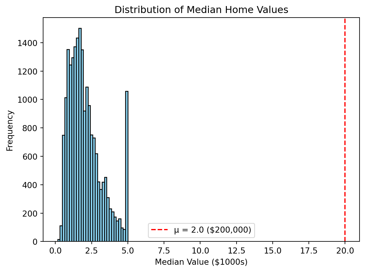

Notice how most homes cluster below the hypothesized mean value, shown by the red dashed line at μ = 2.0 ($200,000).
Most home fall to the left of this line, showing that the actual mean is significantly higher than $200,000, which is consistent with the t-test result
If the data were not normally distributed, meaning the data was skewed or had outliers, we’d use the Wilcoxon Signed-Rank Test instead.
The Wilcoxon Signed-Rank Test compares the median of the sample to a hypothesized value.
$H_0$: median home value = $200{,}000
$H_1$: median home value $\ne$ $200{,}000

from scipy.stats import wilcoxon

prices = housing["medv"].dropna()

w_stat, p_value = wilcoxon(prices - 2.0, alternative="two-sided")
w_stat, p_value

(np.float64(99446113.5), np.float64(1.1542596775842864e-14))

alpha = 0.05
if p_value < alpha:
    print(f"Reject $H_0$ (p = {p_value:.4f}) → Median home value differs from $200,000.")
else:
    print(f"Fail to reject $H_0$ (p = {p_value:.4f}) → No evidence of a difference from $200,000.")

Reject $H_0$ (p = 0.0000) → Median home value differs from $200,000.

wilcoxon() tests whether the median of the sample differs from a hypothesized value
alternative=“twosided” checks for any difference

7.8.7 Two Sample T-Test

A two-sample t-test (also called an independent samples t-test) is used to compare the means of two independent groups to see if they’re statistically different from each other.
Here, we test whether median home values differ between high-income and low-income neighborhoods, based on medinc (median income).
Let:
- Group 1: tracts with medinc above the median (“high income”)
- Group 2: tracts with medinc at or below the median (“low income”)
Hypotheses:
- $H_0: \mu_{\text{high}} = \mu_{\text{low}}$
- $H_1: \mu_{\text{high}} \ne \mu_{\text{low}}$

housing = housing.rename(columns={
    "MedInc": "medinc",
    "MedHouseVal": "medv",
})

income_median = housing["medinc"].median()
high_income = housing[housing["medinc"] > income_median]["medv"].dropna()
low_income = housing[housing["medinc"] <= income_median]["medv"].dropna()

t_stat, p_value = stats.ttest_ind(high_income, low_income, equal_var=False)
print(f"T-statistic: {t_stat:.3f}, P-value: {p_value:.4f}")

T-statistic: 86.363, P-value: 0.0000

alpha = 0.05
if p_value < alpha:
    print(f"Reject $H_0 (p = {p_value:.4f}) → Mean home values differ.")
else:
    print(f"Fail to reject $H_0 (p = {p_value:.4f}) → No difference in mean home values.")

Reject $H_0 (p = 0.0000) → Mean home values differ.

ttest_ind() compares means of two independent groups
equal_var=False: Welch’s t-test version, which doesn’t assume equal variances
We can visualize these differences using boxplots
The boxes represent interquartile ranges, so if they barely overlap that’s a visual clue of statistical difference

housing["income_group"] = np.where(housing["medinc"] > income_median,
"High income",
"Low income")

sns.boxplot(x="income_group", y="medv", data=housing)
plt.title("Median Home Values – High vs. Low Income Neighborhoods")
plt.xlabel("Income Group")
plt.ylabel("Median Home Value (medv)")
plt.show()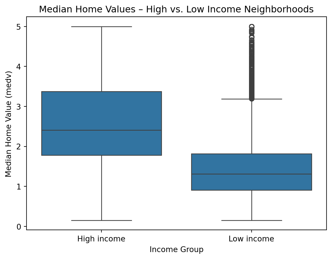

If the data don’t meet the t-test assumptions (normality, equal variance), we use the Mann-Whitney U test between two groups
In this case, we will test whether the distributions of median home values differ for houses near versus away from the Charles River
$H_0$: the distributions of medv are the same in high- and low-income tracts
$H_1$: the distributions differ

from scipy import stats
stat, p_value = stats.mannwhitneyu(high_income, low_income, alternative="two-sided")

print(f"Mann-Whitney U statistic: {stat:.3f}, P-value: {p_value:.4f}")

alpha = 0.05
if p_value < alpha:
    print(f"Reject $H_0$ (p = {p_value:.4f}) → "f"Median home values differ between income groups.")
else:
    print(f"Fail to reject $H_0$ (p = {p_value:.4f}) → " f"No difference in median home values by income group.")

Mann-Whitney U statistic: 87648425.000, P-value: 0.0000
Reject $H_0$ (p = 0.0000) → Median home values differ between income groups.

7.8.8 ANOVA

ANOVA stands for Analysis of Variance
It’s a statistical method used to compare the means of three or more groups to determine whether at least one of them is significantly different from the others.
Here, we’ll compare average home values across income quartiles based on medinc. levels of highway accessibility (rad).
$H_0$: all income quartiles have the same mean home value
$H_1$: at least one quartile mean differs

housing["income_quartile"] = pd.qcut(
housing["medinc"],
q=4,
labels=["Q1 (lowest)", "Q2", "Q3", "Q4 (highest)"]
)

groups = [group["medv"].dropna() for _, group in housing.groupby("income_quartile")]

f_stat, p_value = stats.f_oneway(*groups)

print(f"F-statistic: {f_stat:.3f}, P-value: {p_value:.4f}")

alpha = 0.05
if p_value < alpha:
    print(f"Reject $H_0$ (p = {p_value:.4f}) → " f"Mean home values differ across income quartiles.")
else:
    print(f"Fail to reject $H_0$ (p = {p_value:.4f}) → " f"No difference in mean home values across income quartiles.")

F-statistic: 4277.066, P-value: 0.0000
Reject $H_0$ (p = 0.0000) → Mean home values differ across income quartiles.

/var/folders/cq/5ysgnwfn7c3g0h46xyzvpj800000gn/T/ipykernel_8983/3497753232.py:7: FutureWarning:

The default of observed=False is deprecated and will be changed to True in a future version of pandas. Pass observed=False to retain current behavior or observed=True to adopt the future default and silence this warning.

f_oneway() performs the one-way ANOVA test
To see this visually:

sns.boxplot(x="income_quartile", y="medv", data=housing)
plt.title("Home Values Across Income Quartiles")
plt.xlabel("Income Quartile (medinc)")
plt.ylabel("Median Home Value (medv)")
plt.show()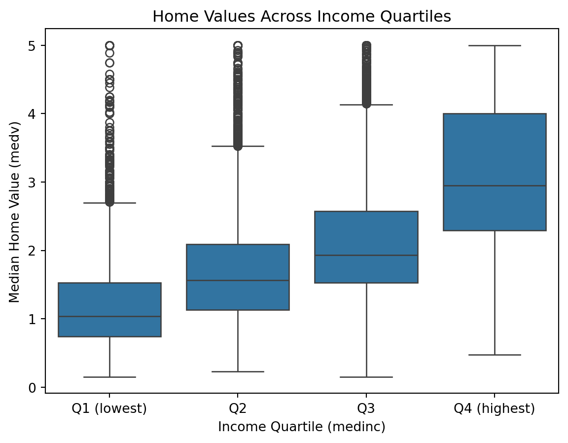

The Kruskal–Wallis test is a nonparametric alternative to one-way ANOVA.
It’s used when the normality assumption is violated or the data contain outliers.
$H_0$: the distributions of medv are the same across all income quartiles
$H_1$: at least one distribution differs

groups = [group["medv"].dropna() for _, group in housing.groupby("income_quartile")]

h_stat, p_value = stats.kruskal(*groups)

print(f"H-statistic: {h_stat:.3f}, P-value: {p_value:.4f}")

alpha = 0.05
if p_value < alpha:
    print(f"Reject $H_0$ (p = {p_value:.4f}) → " f"Median home values differ across income quartiles.")
else:
    print(f"Fail to reject $H_0$ (p = {p_value:.4f}) → "f"No difference in median home values across income quartiles.")

H-statistic: 8726.603, P-value: 0.0000
Reject $H_0$ (p = 0.0000) → Median home values differ across income quartiles.

/var/folders/cq/5ysgnwfn7c3g0h46xyzvpj800000gn/T/ipykernel_8983/3871825430.py:1: FutureWarning:

The default of observed=False is deprecated and will be changed to True in a future version of pandas. Pass observed=False to retain current behavior or observed=True to adopt the future default and silence this warning.

7.8.9 Chi-Square Test of Independence

The Chi-Square Test of Independence checks whether two categorical variables are related or independent of each other.
It’s a nonparametric test, meaning it doesn’t assume normality or equal variances.
We’ll test whether income level is associated with house age category.

housing = housing.rename(columns={
    "MedInc": "medinc",
    "HouseAge": "houseage"
})

income_median = housing["medinc"].median()
age_median    = housing["houseage"].median()

housing["high_income"] = np.where(housing["medinc"] > income_median, 1, 0)
housing["old_house"]   = np.where(housing["houseage"] > age_median, 1, 0)

Hypotheses:
- $H_0$: income level and house age category are independent
- $H_1$: there is an association between income level and house age

table = pd.crosstab(housing["high_income"], housing["old_house"])

chi2, p_value, dof, expected = stats.chi2_contingency(table)

print(f"Chi2 Statistic: {chi2:.3f}, P-value: {p_value:.4f}, Degrees of Freedom: {dof}")

alpha = 0.05
if p_value < alpha:
    print(f"Reject $H_0$ (p = {p_value:.4f}) → " f"There is a significant association between income level and house age.")
else:
    print(f"Fail to reject $H_0$ (p = {p_value:.4f}) → " f"No significant association between income level and house age.")

Chi2 Statistic: 140.180, P-value: 0.0000, Degrees of Freedom: 1
Reject $H_0$ (p = 0.0000) → There is a significant association between income level and house age.

pd.crosstab() creates a contingency table
chi2_contingency() tests independence of two categorical variables
Visual

sns.countplot(x="old_house", hue="high_income", data=housing)
plt.title("House Age Category by Income Level")
plt.xlabel("Old House (1 = older than median age)")
plt.ylabel("Count of Tracts")
plt.legend(title="High Income (1 = above median medinc)")
plt.show()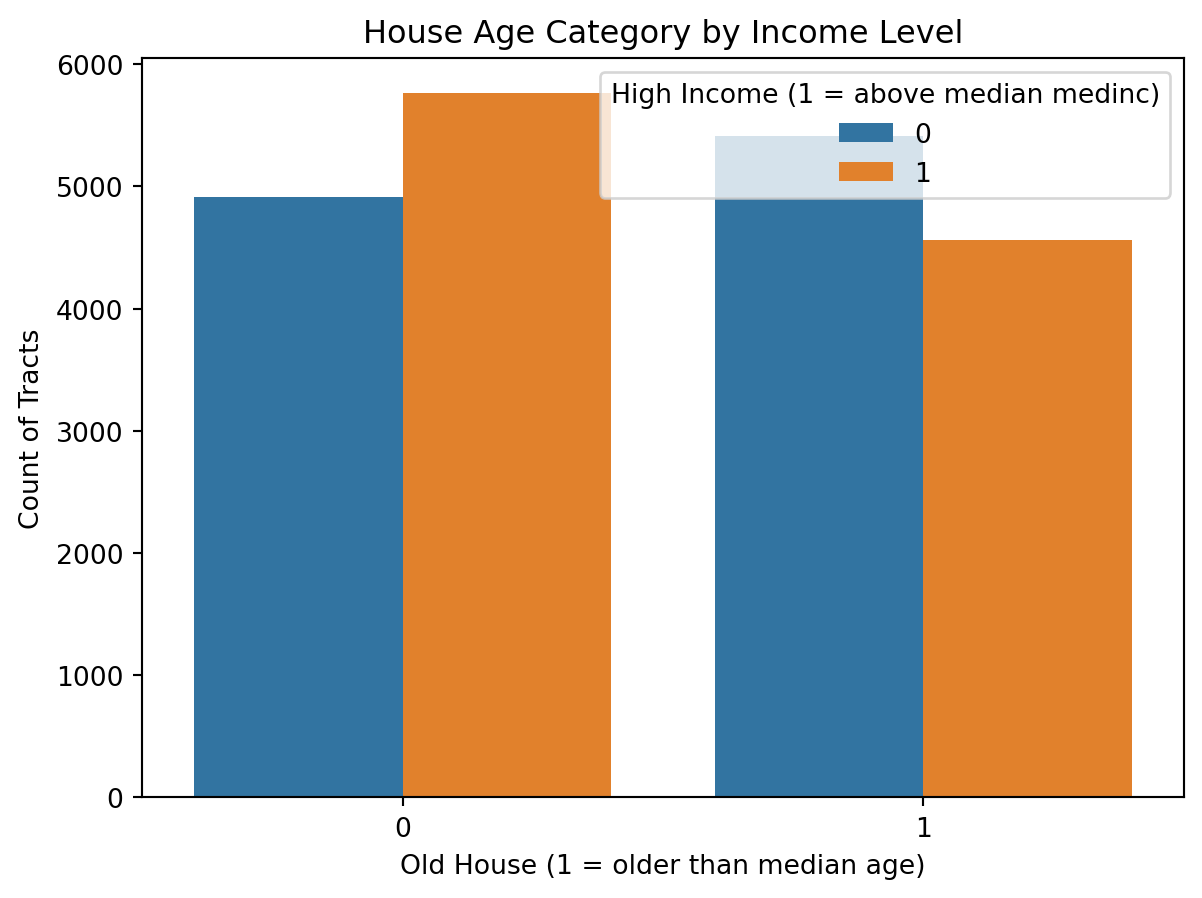

Chi-square tests are great for frequency data, think of them as testing whether “categories are distributed as expected”

7.8.10 Proportion Test

A proportion test is used to compare observed proportions to a hypothesized proportion or between two groups.
Useful for categorical yes/no variables
Suppose we define high-income neighborhoods as those with medinc ≥ 5.0 (median income ≥ $50,000 in this dataset’s units).
$H_0: p = p_0 = 0.30$ (30% of tracts are high income)
$H_1: p \ne p_0$ (the true proportion differs from 30%)

from statsmodels.stats.proportion import proportions_ztest

high_income_flag = housing["medinc"] >= 5.0
count = high_income_flag.sum()
nobs = len(housing)
p0 = 0.30

stat, p_value = proportions_ztest(count, nobs, value=p0, alternative="two-sided")
print(f"Z-statistic: {stat:.3f}, P-value: {p_value:.4f}")

alpha = 0.05
if p_value < alpha:
    print("Reject $H_0$ → The proportion of high-income tracts differs from 30%.")
else:
    print("Fail to reject $H_0$ → No significant difference from 30%.")

Z-statistic: -28.351, P-value: 0.0000
Reject $H_0$ → The proportion of high-income tracts differs from 30%.

nobs is the total homes
p0 is the hypothesized proportionn
proportions_ztest() is the z-test for proportions (like t-test but for percentages)

7.8.11 Correlation Test

The Correlation Test measures the strength and direction of the relationship between two continuous variables.
$r$ close to $+1$ means a strong correlation
$r$ close to $0$ means little or no correlation
$r$ close to $-1$ means a strong negative correlation
Here, we test whether the average number of rooms per dwelling (averooms) is linearly related to median home value (medv).
H$H_0: \rho = 0$ (no linear correlation)
$H_1: \rho \ne 0$ (a significant linear correlation exists)

x = housing["averooms"]
y = housing["medv"]

corr, p_value = stats.pearsonr(x, y)

print(f"Correlation coefficient (r): {corr:.3f}, P-value: {p_value:.4f}")

alpha = 0.05
if p_value < alpha:
    print(f"Reject $H_0$ (p = {p_value:.4f}) → Significant linear correlation.")
else:
    print(f"Fail to reject $H_0$ (p = {p_value:.4f}) → No significant linear correlation.")

Correlation coefficient (r): 0.152, P-value: 0.0000
Reject $H_0$ (p = 0.0000) → Significant linear correlation.

Scatterplot for visualization

sns.scatterplot(x=housing["averooms"], y=housing["medv"], alpha=0.4)
plt.title("Average Rooms vs. Median Home Value")
plt.xlabel("Average Number of Rooms per Dwelling (averooms)")
plt.ylabel("Median Home Value (medv)")
plt.show()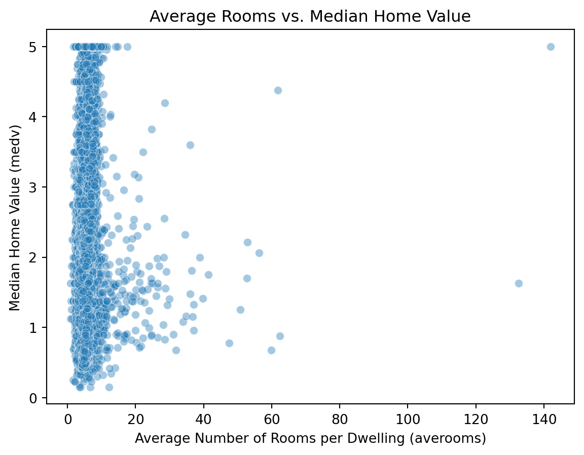

The Spearman correlation coefficient $\rho$ measures the strength and direction of a monotonic relationship between two continuous variables.
Unlike Pearson’s correlation, it doesn’t assume normality or a linear relationship.
$H_0: \rho = 0$ (no monotonic relationship)
$H_1: \rho \ne 0$ (a monotonic relationship exists)

x = housing["averooms"]
y = housing["medv"]

rho, p_value = stats.spearmanr(x, y)

print(f"Spearman’s rho: {rho:.3f}, P-value: {p_value:.4f}")

alpha = 0.05
if p_value < alpha:
    print(f"Reject $H_0$ (p = {p_value:.4f}) → Significant monotonic relationship.")
else:
    print(f"Fail to reject $H_0$ (p = {p_value:.4f}) → No significant monotonic relationship.")

Spearman’s rho: 0.263, P-value: 0.0000
Reject $H_0$ (p = 0.0000) → Significant monotonic relationship.

7.8.12 Summary of Tests

Each statisical test corresponds to a specific research question type:

data = {
    "Test": [
        "One-sample t-test",
        "Wilcoxon Signed-Rank Test",
        "Two-sample t-test",
        "Mann–Whitney U Test",
        "ANOVA",
        "Kruskal–Wallis Test",
        "Chi-Square Test",
        "Proportion Test (z-test)",
        "Pearson Correlation",
        "Spearman Correlation"
    ],
    "Purpose": [
        "Compare sample mean to a known value",
        "Nonparametric alternative to one-sample t-test",
        "Compare means between two independent groups",
        "Nonparametric alternative to two-sample t-test",
        "Compare means across 3+ groups",
        "Nonparametric alternative to ANOVA",
        "Test association between categorical variables",
        "Compare observed vs expected proportions",
        "Measure linear relationship between two continuous variables",
        "Measure monotonic relationship between two continuous variables"
    ],
    "Example": [
        "Avg home value vs $200k",
        "Median home value vs $200k",
        "High- vs low-income neighborhoods",
        "High- vs low-income neighborhoods",
        "Home values across income quartiles",
        "Home values across income quartiles",
        "Income level vs house age category",
        "Proportion of high-income tracts = 30%",
        "Average rooms vs home value",
        "Average rooms vs home value"
    ],
    "Interpretation": [
        "Is mean ≠ hypothesized value?",
        "Is median ≠ hypothesized value?",
        "Difference in group means",
        "Difference in group medians",
        "At least one mean differs",
        "At least one median differs",
        "Are the variables independent?",
        "Is the proportion different from expected?",
        "Is there a linear correlation?",
        "Is there a monotonic correlation?"
    ]
}

df = pd.DataFrame(data)
df

	Test	Purpose	Example	Interpretation
0	One-sample t-test	Compare sample mean to a known value	Avg home value vs $200k	Is mean ≠ hypothesized value?
1	Wilcoxon Signed-Rank Test	Nonparametric alternative to one-sample t-test	Median home value vs $200k	Is median ≠ hypothesized value?
2	Two-sample t-test	Compare means between two independent groups	High- vs low-income neighborhoods	Difference in group means
3	Mann–Whitney U Test	Nonparametric alternative to two-sample t-test	High- vs low-income neighborhoods	Difference in group medians
4	ANOVA	Compare means across 3+ groups	Home values across income quartiles	At least one mean differs
5	Kruskal–Wallis Test	Nonparametric alternative to ANOVA	Home values across income quartiles	At least one median differs
6	Chi-Square Test	Test association between categorical variables	Income level vs house age category	Are the variables independent?
7	Proportion Test (z-test)	Compare observed vs expected proportions	Proportion of high-income tracts = 30%	Is the proportion different from expected?
8	Pearson Correlation	Measure linear relationship between two contin...	Average rooms vs home value	Is there a linear correlation?
9	Spearman Correlation	Measure monotonic relationship between two con...	Average rooms vs home value	Is there a monotonic correlation?

7.8.13 Discussions and Takeaways

Check assumptions: normality, independence, equal variance.
Use nonparametric methods when assumptions fail.
Statistical significance ≠ practical importance.
Clear hypotheses + clean data = valid conclusions.

7.8.14 Further Readings

SciPy.stats Documentation: https://docs.scipy.org/doc/scipy/reference/stats.html
“Practical Statistics for Data Scientists” — Bruce & Gedeck
“Think Stats” by Allen B. Downey