8  Regression Models

Regression is a fundamental tool in data science and statistics for modeling relationships between variables. It provides a framework to explain how a response variable changes when one or more explanatory variables vary, and it serves as a foundation for prediction, interpretation, and decision making. Regression models are used in a wide range of applications, from estimating the effect of education on income to predicting housing prices based on property characteristics.

8.1 Introduction

This chapter introduces regression through a unified set of examples using the Ames Housing dataset. The dataset contains detailed information about housing sales in Ames, Iowa. It has become a popular benchmark for regression tasks, replacing the older Boston Housing dataset due to its larger size and richer set of features. Throughout the chapter, we will use this dataset to illustrate concepts of regression modeling, including model formulation, fitting, diagnosis, and extensions such as regularization, GLM, and GAM. Because many variables in the dataset record absence with NA (for example, NA in the alley variable indicates no alley access), careful preprocessing is required before modeling.

8.1.1 Ames Housing Data Cleaning

The Ames housing data will be used for illustration, but it requires careful preprocessing. A distinctive feature of this dataset is that many NA values do not represent missing information but instead denote the absence of a feature. Treating them as missing would discard useful signals, so they should be recoded explicitly.

First, we retrieve the data to ensure reproducibility.

import openml
import pandas as pd

# Load Ames Housing dataset (OpenML ID 42165)
dataset = openml.datasets.get_dataset(42165)
df, *_ = dataset.get_data()

For categorical variables, NA often means that the property does not have the feature. For example, Alley is NA when no alley access exists, FireplaceQu is NA when no fireplace is present, and PoolQC is NA when the house does not have a pool. In these cases, NA should be replaced with an explicit category such as “None.”

none_cols = [
    "Alley", "FireplaceQu", "PoolQC", "Fence", "MiscFeature",
    "GarageType", "GarageFinish", "GarageQual", "GarageCond",
    "BsmtQual", "BsmtCond", "BsmtExposure", "BsmtFinType1",
    "BsmtFinType2", "MasVnrType"
]
for col in none_cols:
    df[col] = df[col].fillna("None")

For numeric variables, NA may also indicate absence. Examples include GarageCars, GarageArea, and basement square footage variables. When no garage or basement is present, the correct encoding is zero. Thus, these columns should be filled with 0 rather than treated as missing.

zero_cols = [
    "GarageCars", "GarageArea",
    "BsmtFinSF1", "BsmtFinSF2", "BsmtUnfSF",
    "TotalBsmtSF", "BsmtFullBath", "BsmtHalfBath",
    "MasVnrArea"
]
for col in zero_cols:
    df[col] = df[col].fillna(0)

Finally, some variables contain genuinely missing data. A common example is LotFrontage, which records the linear feet of street connected to a property. Here NA values reflect unavailable measurements. These can be imputed using summary statistics such as the median or by more advanced methods if desired.

df["LotFrontage"] = df["LotFrontage"].fillna(df["LotFrontage"].median())

This structured cleaning step ensures that absence is distinguished from missingness, numeric zero values are meaningful, and true missing values are handled appropriately. Only after this preparation is the dataset ready for modeling.

8.2 Linear Regression Model

The starting point of regression analysis is the specification of a model that links a response variable to one or more explanatory variables. In the simplest form, the relationship is described by a linear function plus an error term:

\[ Y_i = \beta_0 + \beta_1 X_{i1} + \cdots + \beta_p X_{ip} + \varepsilon_i, \]

where \(Y_i\) is the response for observation \(i\), \(X_{ij}\) are the explanatory variables, \(\beta_j\) are unknown coefficients, and \(\\varepsilon_i\) is a random error term. The model asserts that systematic variation in the response is captured by a linear combination of predictors, while unsystematic variation is left to the error.

For linear regression to yield valid estimates and inference, several assumptions are commonly made. The form of the mean function is assumed linear in parameters. The error terms are assumed to have mean zero and constant variance, and to be independent across observations. When sample sizes are small, normality of the errors is sometimes assumed to justify exact inference. With larger samples, asymptotic results make this assumption less critical, and estimation of coefficients by least squares does not require it. Finally, explanatory variables should not be perfectly collinear. These assumptions guide model fitting and motivate the diagnostic checks that follow.

8.2.1 Fitting

Fitting a regression model means finding estimates of the coefficients that make the model align with observed data. The most common approach is ordinary least squares, which minimizes the sum of squared residuals:

\[ L(\beta) = \sum_{i=1}^n (Y_i - \beta_0 - \beta_1 X_{i1} - \cdots - \beta_p X_{ip})^2. \]

Here \(L(\beta)\) is the loss function, measuring how far predictions are from observed responses. Minimizing this quadratic loss yields closed form solutions for the coefficient estimates when predictors are not perfectly collinear. Computationally, this involves solving the normal equations or using matrix decompositions such as QR or singular value decomposition, which provide stable and efficient solutions.

This framework also sets the stage for extensions. By modifying the loss function to include penalty terms, one obtains regularization methods such as ridge regression or the lasso. The optimization remains similar in spirit but balances data fit with model complexity. Later sections will show how these modifications improve prediction and interpretability when many predictors are involved.

Housing prices are highly skewed, with a long right tail. To stabilize variance and make the model fit better, it is common to use the log of SalePrice as the response:

\[ Y_i = \log(\text{SalePrice}_i). \]

We add this transformed response to the dataset.

import numpy as np

df["LogPrice"] = np.log(df["SalePrice"])

Many studies and analyses of the Ames data have found certain variables to be consistently important for predicting sale price. These include OverallQual (overall material and finish quality), GrLivArea (above- ground living area), GarageCars (garage capacity), TotalBsmtSF (total basement area), YearBuilt (construction year), FullBath (number of full bathrooms), and KitchenQual (kitchen quality). We will focus on these predictors to illustrate model fitting.

Instead of manually creating dummy variables, we can use the formula API from statsmodels, which handles categorical predictors internally.

import statsmodels.formula.api as smf

formula = (
    "LogPrice ~ OverallQual + GrLivArea + GarageCars + "
    "TotalBsmtSF + YearBuilt + FullBath + C(KitchenQual)"
)

We then fit the regression model directly with the formula.

model = smf.ols(formula, data=df).fit()

Finally, we examine the regression results, which highlight the most important predictors of log sale price.

model.summary()

OLS Regression Results

Dep. Variable:	LogPrice	R-squared:	0.819
Model:	OLS	Adj. R-squared:	0.818
Method:	Least Squares	F-statistic:	727.5
Date:	Tue, 18 Nov 2025	Prob (F-statistic):	0.00
Time:	15:23:41	Log-Likelihood:	515.19
No. Observations:	1460	AIC:	-1010.
Df Residuals:	1450	BIC:	-957.5
Df Model:	9
Covariance Type:	nonrobust

	coef	std err	t	P>|t|	[0.025	0.975]
Intercept	6.8033	0.419	16.219	0.000	5.980	7.626
C(KitchenQual)[T.Fa]	-0.2146	0.037	-5.780	0.000	-0.287	-0.142
C(KitchenQual)[T.Gd]	-0.0653	0.020	-3.257	0.001	-0.105	-0.026
C(KitchenQual)[T.TA]	-0.1348	0.023	-5.931	0.000	-0.179	-0.090
OverallQual	0.0882	0.006	15.841	0.000	0.077	0.099
GrLivArea	0.0002	1.34e-05	17.987	0.000	0.000	0.000
GarageCars	0.0822	0.008	10.056	0.000	0.066	0.098
TotalBsmtSF	0.0001	1.28e-05	9.134	0.000	9.2e-05	0.000
YearBuilt	0.0021	0.000	9.686	0.000	0.002	0.003
FullBath	-0.0087	0.012	-0.727	0.467	-0.032	0.015

Omnibus:	962.926	Durbin-Watson:	1.990
Prob(Omnibus):	0.000	Jarque-Bera (JB):	36561.376
Skew:	-2.522	Prob(JB):	0.00
Kurtosis:	26.991	Cond. No.	2.57e+05

Notes:
[1] Standard Errors assume that the covariance matrix of the errors is correctly specified.
[2] The condition number is large, 2.57e+05. This might indicate that there are
strong multicollinearity or other numerical problems.

The output gives estimated coefficients, standard errors, and measures of fit. At this stage, several questions naturally arise:

• How should we interpret a coefficient when the outcome is on the log scale? For instance, what does a one-unit increase in OverallQual imply for expected sale price?
• How do we compare the importance of variables measured on different scales, such as square footage and construction year?
• What role do categorical variables like KitchenQual play, and how do we interpret their dummy coefficients relative to the baseline?
• Which predictors are statistically significant, and does significance necessarily imply practical importance?
• How well does the model explain variation in housing prices, and what limitations might remain?

These questions guide us in interpreting the fitted model and connect directly to the diagnostic checks discussed in the next section.

8.2.2 Diagnosis

Once a regression model has been fitted, it is essential to examine whether the underlying assumptions hold and whether the model provides a useful description of the data. Diagnostics help identify potential problems such as non-linearity, heteroscedasticity, influential points, and violations of independence.

The first step is to examine residuals, defined as the difference between observed and fitted values:

\[ \hat{\varepsilon}_i = Y_i - \hat{Y}_i. \]

Plotting residuals against fitted values reveals whether variance is constant and whether systematic patterns remain.

import matplotlib.pyplot as plt

fitted_vals = model.fittedvalues
residuals = model.resid

plt.scatter(fitted_vals, residuals, alpha=0.5)
plt.axhline(0, color="red", linestyle="--")
plt.xlabel("Fitted values")
plt.ylabel("Residuals")
plt.title("Residuals vs Fitted")
plt.show()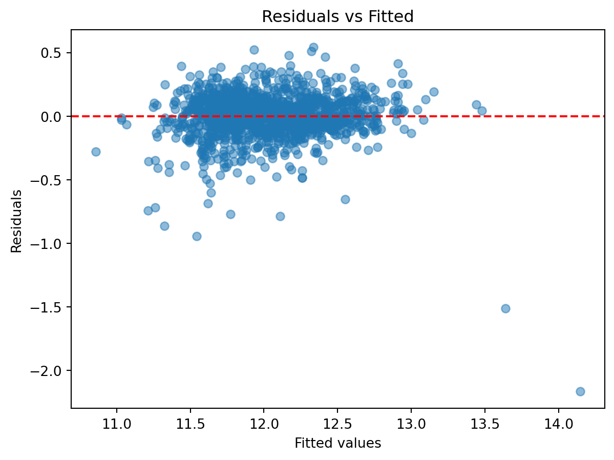

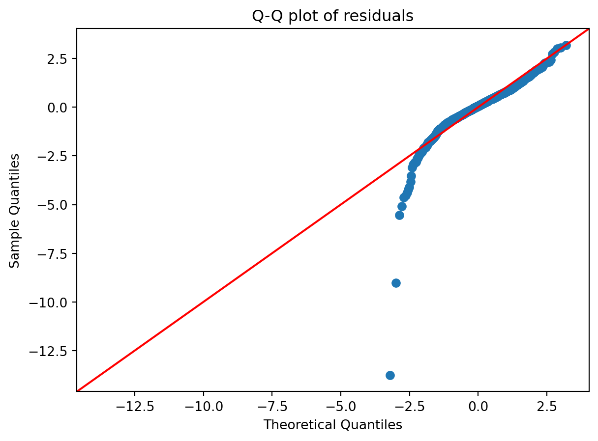
Another check is the distribution of residuals. A histogram or Q-Q plot can indicate whether residuals are approximately normal, which is most relevant for inference in small samples.

plt.hist(residuals, bins=30, edgecolor="black")
plt.xlabel("Residuals")
plt.title("Histogram of residuals")
plt.show()

influence = model.get_influence()
std_resid = influence.resid_studentized_internal

import statsmodels.api as sm
sm.qqplot(std_resid, line="45")
plt.title("Q-Q plot of residuals")
plt.show()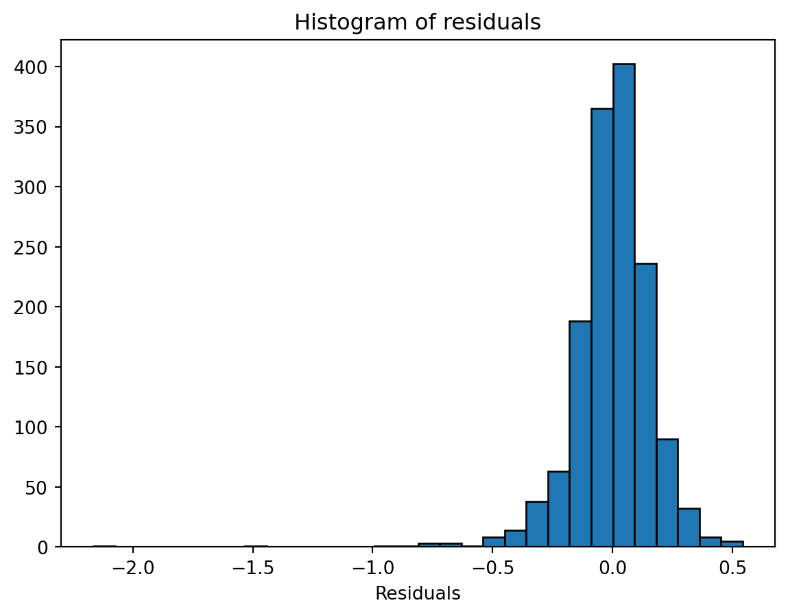

Influential observations can distort regression results. Leverage and Cook’s distance are standard measures to detect such points.

cooks = influence.cooks_distance[0]

plt.scatter(fitted_vals, cooks, alpha=0.5)
plt.xlabel("Fitted values")
plt.ylabel("Cook's distance")
plt.title("Influence diagnostics")
plt.show()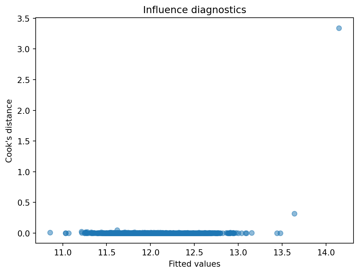

Key questions to raise at this stage are:

• Do residuals appear randomly scattered, suggesting the linear model is adequate?
• Is there evidence of non-constant variance or other systematic patterns?
• Are residuals approximately normal, and does this matter given the sample size?
• Which points exert disproportionate influence on the fitted model?

These diagnostic tools guide improvements, such as transformations, adding interaction terms, or considering alternative modeling approaches.

8.3 Regularized Regression

8.3.1 Motivation

Ordinary least squares can perform poorly when there are many predictors or when predictors are highly correlated. In such cases, estimated coefficients become unstable and prediction accuracy suffers. Regularization introduces penalties on the size of coefficients, leading to simpler and more robust models.

To illustrate, we return to the Ames data. Suppose we fit a model with a large set of predictors. Ordinary least squares will attempt to explain every fluctuation in the data, potentially overfitting. A regularized approach reduces this risk by shrinking coefficients, improving out-of-sample prediction.

8.3.2 Formulation

The penalized regression framework modifies the least squares objective:

\[ L(\beta) = \sum_{i=1}^n (Y_i - X_i^\top \beta)^2 + \lambda P(\beta), \]

where \(P(\beta)\) is a penalty function and \(\lambda\) controls its strength.

For ridge regression the penalty is

\[ P(\beta) = \sum_j \beta_j^2, \]

which shrinks coefficients smoothly toward zero but never sets them exactly to zero. For lasso regression the penalty is

\[ P(\beta) = \sum_j |\beta_j|. \]

Because the absolute value has a sharp corner at zero, lasso can shrink some coefficients exactly to zero. This property allows lasso to perform variable selection and estimation in a single step, producing sparse models in which unimportant predictors are excluded automatically. Elastic net combines both types of penalties.

8.3.3 Algorithms

Ridge regression has a closed-form solution obtained by modifying the normal equations. Lasso and elastic net require iterative algorithms, with coordinate descent being the most widely used. In practice, these algorithms are efficient and scale well to high-dimensional data.

When using scikit-learn, predictors must be numeric. Since the Ames data include categorical variables such as KitchenQual, we need to encode them. We use a OneHotEncoder inside a ColumnTransformer. This transforms categorical variables into binary indicator columns while keeping numeric variables unchanged. The drop="first" option avoids perfect collinearity by omitting one reference category.

from sklearn.preprocessing import StandardScaler
from sklearn.preprocessing import OneHotEncoder
from sklearn.compose import ColumnTransformer
from sklearn.pipeline import Pipeline
from sklearn.linear_model import Ridge, Lasso
from sklearn.model_selection import train_test_split

numeric_features = [
    "OverallQual", "GrLivArea", "GarageCars",
    "TotalBsmtSF", "YearBuilt", "FullBath"
]
categorical_features = ["KitchenQual"]

preprocessor = ColumnTransformer(
    transformers=[
        ("num", StandardScaler(), numeric_features),
        ("cat", OneHotEncoder(drop="first"), categorical_features)
    ]
)

X = df[numeric_features + categorical_features]
y = df["LogPrice"]

X_train, X_test, y_train, y_test = train_test_split(
    X, y, test_size=0.3, random_state=42
)

ridge = Pipeline(steps=[
    ("preprocessor", preprocessor),
    ("model", Ridge(alpha=10))
]).fit(X_train, y_train)

lasso = Pipeline(steps=[
    ("preprocessor", preprocessor),
    ("model", Lasso(alpha=0.1))
]).fit(X_train, y_train)

8.3.4 Solution Paths

As the penalty parameter \(\lambda\) decreases, the behavior of coefficients changes. Ridge coefficients approach ordinary least squares estimates, while lasso coefficients enter the model sequentially, illustrating variable selection.

Because predictors must be on the same scale for a fair comparison, it is important to standardize the numeric variables before computing the lasso path. Without standardization, some coefficients can appear flat or dominate others due to differences in scale.

In our Ames example, we have six numeric predictors and three dummy variables for KitchenQual (since one category was dropped). This means we are estimating nine coefficients in total, excluding the intercept. All nine should appear in the solution path once variables are properly scaled.

from sklearn.preprocessing import StandardScaler
from sklearn.linear_model import lasso_path
import numpy as np

# Standardized predictors
X_proc = preprocessor.fit_transform(X_train)
scaler = StandardScaler(with_mean=False)
X_proc_std = scaler.fit_transform(X_proc)

# Compute lambda_max
n_samples = X_proc_std.shape[0]
lambda_max = np.max(np.abs(X_proc_std.T @ y_train)) / n_samples

# Define a grid of lambda values
alphas = np.logspace(np.log10(lambda_max), -3, 50)

# Compute solution path
alphas, coefs, _ = lasso_path(X_proc_std, y_train, alphas=alphas)

plt.plot(alphas, coefs.T)
plt.xscale("log")
plt.xlabel("Lambda")
plt.ylabel("Coefficients")
plt.title("Lasso solution paths starting at lambda_max")
plt.show()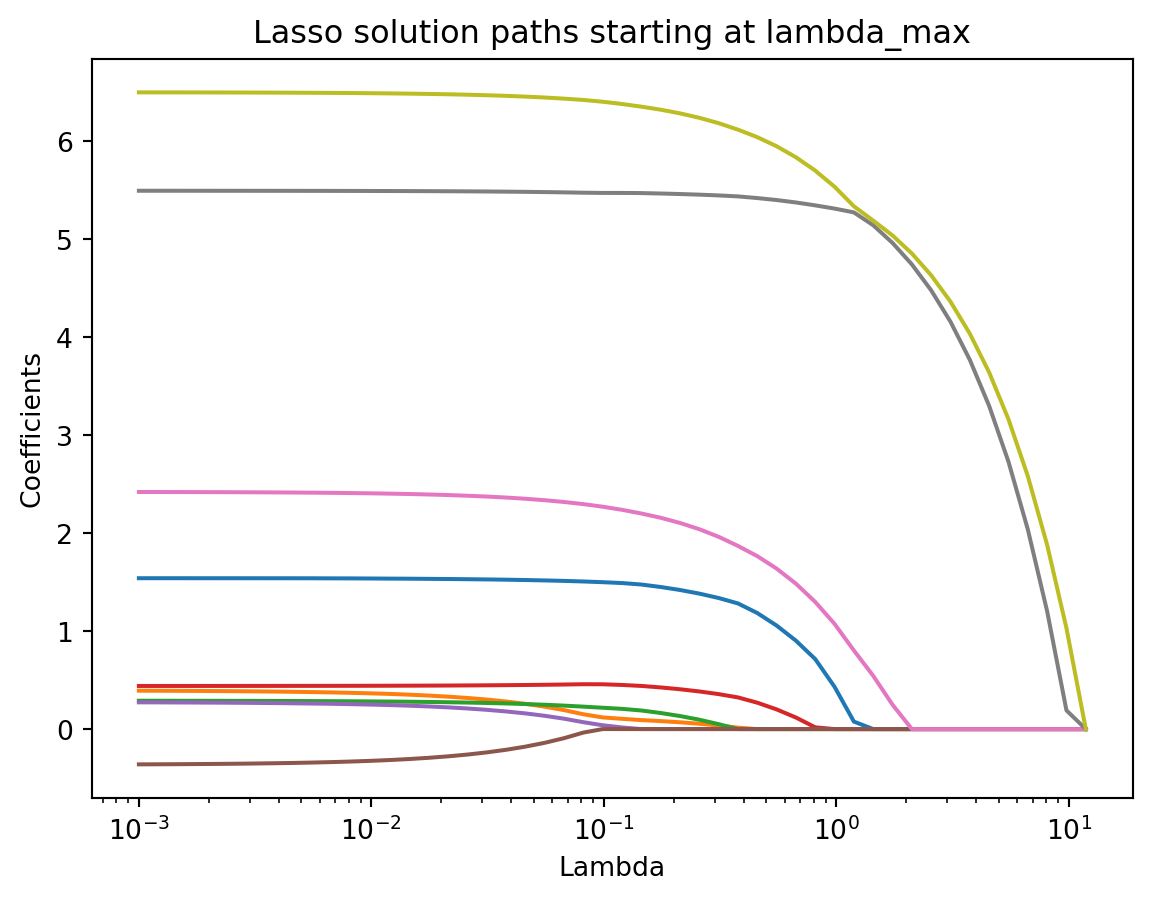

This plot reveals how each coefficient evolves as \(\lambda\) changes. At large values of \(\lambda\), coefficients are shrunk close to zero. As \(\lambda\) decreases, more predictors enter the model. The intercept is not included in the path and should be ignored when interpreting these curves.

8.3.5 Tuning Parameter Selection

Choosing \(\lambda\) is critical. Too large, and the model is oversmoothed; too small, and the penalty has little effect. This parameter controls the trade-off between model fit and complexity:

• When \(\lambda = 0\), the model reduces to the unpenalized regression.
• As \(\lambda \to \infty\), coefficients shrink toward zero, increasing bias but reducing variance.

Choosing \(\lambda\) appropriately is crucial. A general principle is to define a selection criterion \(C(\lambda)\), which measures the predictive or explanatory performance of the fitted model, and then select \(\hat{\lambda} = \arg\min_{\lambda} C(\lambda)\).

Common criteria:

• \(R^2\) on a validation set: select \(\lambda\) that maximizes explained variance.
• Information criteria (AIC, BIC): less common in practice for penalized regression.
• Cross-validation (CV): partition data, fit on training folds, evaluate on holdout fold, average prediction error across folds.

The grid of candidate values is not arbitrary:

• Maximum value:

  \[ \lambda_{\max} = \max_j \tfrac{1}{n} |x_j^\top y|, \]

  with standardized predictors. At this level, all coefficients are zero.

• Minimum value: \[ \lambda_{\min} = \epsilon \cdot \lambda_{\max}, \] with \(\epsilon = 10^{-3}\) if \(n > p\) and \(\epsilon = 10^{-2}\) otherwise.

• Grid: values are log-spaced between \(\lambda_{\max}\) and \(\lambda_{\min}\) (default 100 points in scikit-learn).

In the Ames example, we can use \(k\)-fold cross-validation to evaluate ridge and lasso models.

from sklearn.linear_model import LassoCV
from sklearn.pipeline import Pipeline
from sklearn.model_selection import KFold

# Lasso with 10-fold CV
lasso_cv = LassoCV(
    cv=KFold(n_splits=10, shuffle=True, random_state=123),
    random_state=123
)

# Pipeline with preprocessing + model
pipe = Pipeline(steps=[
    ("preprocessor", preprocessor),
    ("model", lasso_cv)
])

pipe.fit(X, y)

# Selected lambda
best_lambda = pipe.named_steps["model"].alpha_
print("Best lambda (alpha) selected by CV:", best_lambda)

Best lambda (alpha) selected by CV: 0.00032631403363203007

This process identifies the tuning parameter that balances bias and variance most effectively, yielding a model that generalizes well beyond the training data.

8.4 Generalized Linear Models

8.4.1 Introduction

Linear regression is a powerful tool for continuous outcomes under Gaussian assumptions, but many response variables encountered in practice are not continuous or normally distributed. For example, an indicator of whether a house sale price is above the median is binary, the number of bathrooms is a count, and proportions such as the fraction of remodeled homes lie between 0 and 1. Using linear regression in these settings can yield nonsensical predictions (e.g., negative counts or probabilities outside the unit interval).

Generalized linear models (GLMs) extend linear regression to cover a wider range of outcomes. The key idea is to preserve the familiar linear predictor structure, while linking it to the mean of the outcome through a function that reflects the nature of the data. The formal framework was introduced by Nelder & Wedderburn (1972) and remains central in modern statistics. Today, GLMs are viewed more flexibly: the distributional assumption provides a convenient likelihood-based loss function, but in practice one can proceed with quasi-likelihood or even direct loss minimization without strict distributional commitment.

8.4.2 Framework

GLMs extend linear regression by introducing a link function between the linear predictor and the conditional mean of the response. In linear regression we write

\[ Y_i = X_i^\top \beta + \varepsilon_i \]

with mean zero error \(\varepsilon_i\)’s.

The mean is simply \(\mu_i = X_i^\top \beta\). In a GLM, we allow non-Gaussian outcomes by defining

\[ \eta_i = X_i^\top \beta, \quad g(\mu_i) = \eta_i, \]

where \(g(\cdot)\) is a monotone link function, \(\mu_i = \mathbb{E}(Y_i)\), and \(\beta\) are regression coefficients. The coefficients maintain the same interpretation as in linear regression: a one-unit change in a predictor shifts the linear predictor \(\eta_i\) by its coefficient, with an indirect effect on \(\mu_i\) through the link.

The variance of \(Y_i\) depends on the mean: \(\text{Var}(Y_i) = V(\mu_i) \cdot \phi\), where \(V(\cdot)\) is the variance function and \(\phi\) is a dispersion parameter. This structure arises naturally from the exponential family, which provides a unifying framework for GLMs. While exact distributional assumptions can be specified, the mean–variance relationship is often sufficient.

8.4.3 Special Cases

• Logistic regression

  For binary outcomes,

  \[ Y_i \sim \text{Bernoulli}(\mu_i), \qquad g(\mu_i) = \log \frac{\mu_i}{1-\mu_i}. \]

  The coefficient \(\beta_j\) quantifies the log-odds change of success for a one-unit increase in \(x_{ij}\), with other covariates held fixed.

• Poisson regression

  For count data,

  \[ Y_i \sim \text{Poisson}(\mu_i), \qquad g(\mu_i) = \log(\mu_i). \]

  The coefficient \(\beta_j\) is interpreted as the log rate ratio, where \(\exp(\beta_j)\) gives the multiplicative change in expected count for a one-unit increase in \(x_{ij}\).

• Gaussian regression

  For continuous responses,

  \[ Y_i \sim N(\mu_i, \sigma^2), \qquad g(\mu_i) = \mu_i. \]

  The coefficient \(\beta_j\) represents the expected change in the response for a one-unit increase in \(x_{ij}\).

Thus, GLMs preserve the linear predictor while flexibly adapting the link and variance structure to suit binary, count, and continuous data.

8.4.4 Fitting and Diagnosis

Estimation in generalized linear models is typically carried out by maximum likelihood. The parameters \(\beta\) are obtained by solving the score equations, which in practice are computed through numerical optimization. A common algorithm is iteratively reweighted least squares (IRLS), which updates coefficient estimates using weighted least squares until convergence. In Python, functions such as statsmodels.api.GLM or sklearn.linear_model.LogisticRegression implement this estimation automatically, providing coefficient estimates along with standard errors and confidence intervals when applicable.

After fitting a GLM, model adequacy should be checked through diagnostics. Residuals such as deviance residuals or Pearson residuals can reveal lack of fit and highlight influential observations. Goodness of fit can also be assessed with deviance statistics, likelihood ratio tests, or pseudo-\(R^2\) measures. In Python, statsmodels provides methods like .resid_deviance, .resid_pearson, and influence statistics to assess model fit. Visual inspection through residual plots remains a practical tool to detect systematic deviations from model assumptions.

8.4.5 Regularized GLM

Regularization extends generalized linear models by adding a penalty to the log-likelihood, which stabilizes estimation in high-dimensional settings and enables variable selection. The optimization problem can be formulated as

\[ \hat{\beta} = \arg\min_{\beta} \Big\{ -\ell(\beta) + \lambda P(\beta) \Big\}, \]

where \(\ell(\beta)\) is the log-likelihood, \(P(\beta)\) is a penalty function, and \(\lambda\) is a tuning parameter controlling the strength of shrinkage.

Common choices of \(P(\beta)\) include:

• Ridge (\(L_2\)): \(\sum_j \beta_j^2\).
• Lasso (\(L_1\)): \(\sum_j |\beta_j|\).
• Elastic Net: \(\alpha \sum_j |\beta_j| + (1-\alpha)\sum_j \beta_j^2\).

The fitting algorithm typically involves coordinate descent or gradient- based optimization methods, which are efficient for large-scale data and sparse solutions. For example, the glmnet algorithm uses cyclical coordinate descent with warm starts.

Selection of the tuning parameter \(\lambda\) is crucial. A standard approach is cross-validation, where data are split into folds, the model is fitted on training folds for a grid of \(\lambda\) values, and performance is evaluated on validation folds. The \(\lambda\) yielding the lowest prediction error is chosen, sometimes with an additional rule to prefer more parsimonious models (the “one standard error rule”).

In Python, sklearn.linear_model.LogisticRegressionCV or sklearn.linear_model.ElasticNetCV implement these ideas, providing automatic cross-validation for regularized GLMs.

The general workflow for fitting a regularized logistic regression model is:

1. Define predictors and outcome: choose relevant numeric and categorical features, and specify the binary response.
2. Preprocess features: standardize numeric predictors with StandardScaler() and encode categorical predictors with OneHotEncoder().
3. Set up the pipeline: combine preprocessing with the logistic regression model in a unified workflow.
4. Fit with cross-validation: use LogisticRegressionCV with lasso (L1) or elastic net penalties. Cross-validation automatically selects the tuning parameter \(\lambda\).
5. Inspect coefficients: identify which predictors remain with nonzero coefficients, interpreting them as important contributors to the outcome.
6. Evaluate performance: measure predictive accuracy or AUC (see chapter on classification) on a held-out test set to assess generalization.

This structured process ensures stability, interpretability, and good predictive performance when fitting regularized logistic models.

8.4.6 Example: Regularized GLM with Ames Housing Data

We continue with the processed Ames housing dataset (OpenML id 42165) from earlier in the regression chapter. The task is to predict whether a home is “expensive” (above the median sale price) using selected predictors. We fit a logistic regression model with an \(L_1\) (lasso) penalty to enable variable selection.

from sklearn.linear_model import LogisticRegressionCV
from sklearn.pipeline import Pipeline

# Binary outcome: 1 if SalePrice > median
median_price = df["SalePrice"].median()
y = (df["SalePrice"] > median_price).astype(int)

# Logistic regression with L1 penalty and cross-validation
logit_lasso_cv = Pipeline(steps=[
    ("preprocessor", preprocessor),
    ("model", LogisticRegressionCV(
         Cs=20, cv=5, penalty="l1", solver="saga",
         scoring="accuracy", max_iter=5000,
         random_state=0
    ))
])

logit_lasso_cv.fit(X, y)

# Extract selected coefficients
model = logit_lasso_cv.named_steps["model"]
feature_names = (
    numeric_features +
    list(logit_lasso_cv.named_steps["preprocessor"]
        .named_transformers_["cat"]
        .get_feature_names_out(categorical_features))
)

print("Selected coefficients (lasso):")
for name, coef in zip(feature_names, model.coef_[0]):
    print(f"{name}: {coef:.4f}")

print("\nBest C (inverse of lambda):", model.C_[0])

Selected coefficients (lasso):
OverallQual: 1.1998
GrLivArea: 1.6516
GarageCars: 0.6534
TotalBsmtSF: 0.5812
YearBuilt: 0.8845
FullBath: 0.1628
KitchenQual_Fa: -1.2791
KitchenQual_Gd: -0.0467
KitchenQual_TA: -0.9568

Best C (inverse of lambda): 1.623776739188721

This example demonstrates how lasso-penalized logistic regression can be used within the GLM framework. The penalty shrinks coefficients toward zero, with some set exactly to zero if uninformative, thereby improving interpretability and predictive stability.

We can evaluate classification performance by computing the confusion matrix:

from sklearn.metrics import confusion_matrix, ConfusionMatrixDisplay

# Predictions
y_pred = logit_lasso_cv.predict(X)

# Confusion matrix
cm = confusion_matrix(y, y_pred)
disp = ConfusionMatrixDisplay(confusion_matrix=cm,
display_labels=["Not Expensive", "Expensive"])
disp.plot(cmap="Blues")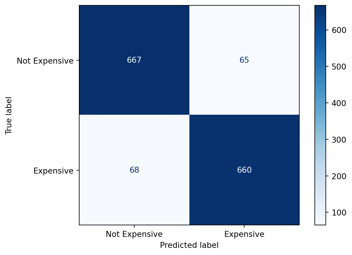

8.5 Spatial Statistical Methods

This section was written by Quinn Saltus, an undergraduate student pursuing a dual degree in Applied Data Analysis and Geograpic Information Systems. They were motivated to write about this topic because they wanted to bridge the geographic and statistical approaches to problem solving.

8.5.1 Introduction

Spatially dependent data can cause problems for standard statistical methods. Independence of errors is an assumption for most commonly-used tools, but if location affects your data, that assumption is untenable. Spatial Statistics can quantify the spatial dependence among data and improve predictive models’ accuracy / statistical rigor.

8.5.2 Dataset

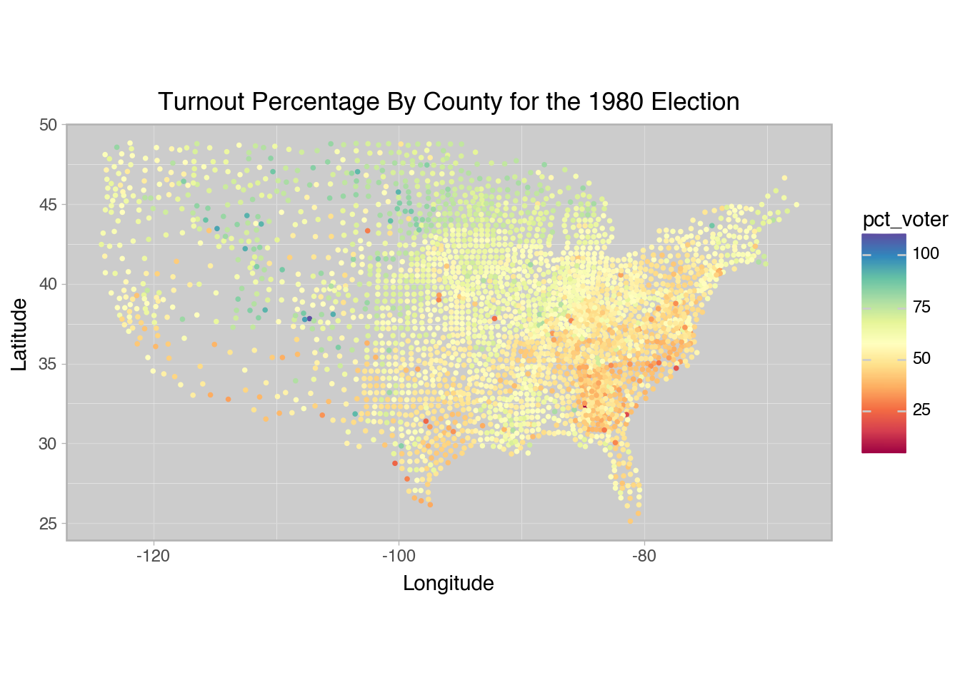
The dataset used in this demonstration is the Turnout by County for the 1980 Election from Pace & Barry (1997).

from plotnine import *
import pandas as pd
import numpy as np
from sklearn.datasets import fetch_openml

dataset = fetch_openml(name='space_ga', version=1)

df = dataset.data
df.columns = df.columns.str.lower()

# convert log-proportion to percentage for ease of understanding
df["pct_voter"] = np.exp(dataset.target) * 100

# convert coordinates to degrees
df["xcoord"] = df["xcoord"] / 10**6
df["ycoord"] = df["ycoord"] / 10**6

(ggplot(df, aes(x="xcoord", y="ycoord", color="pct_voter"))
    + geom_point(size=0.6)
    + scale_color_continuous(cmap_name="Spectral")
    + coord_equal(ratio=1.3)
    + labs(
        title="Turnout Percentage By County for the 1980 Election",
        x="Longitude",
        y="Latitude"
    )
    + theme_light()
    + theme(
        panel_background=element_rect(fill="#cccccc")
    )
)

8.5.3 Libraries

The libraries used are The Python Spatial Analysis Library and PyKrige. These libraries haven’t been used before in this course, so you may need to install them yourself.

pip install pykrige
pip install pysal

I’ll also use Scipy‘s KDTree class, which greatly reduces the amount of computation required to compare data points’ distances. This is important for speed with large datasets.

import libpysal
from scipy.spatial import KDTree
from pysal.explore import esda
import pykrige as pk

8.5.4 Spatial Weights

Standard regression has error terms that are completely random:

\[ Y = \beta X + \epsilon \]

The spatial error model (SEM) formulates residuals as a weighted mean of nearby errors plus a random error term:

\[ Y = \beta X + u, u = \lambda W u + \epsilon \]

With PySAL, we need to precompute the weights matrix \(W\) to give to analysis functions. Inverse square distance is the most popular and will be used here. Other methods like K-Nearest-Neighbors (libpysal.weights.KNN) and Gabriel Graphs (libpysal.weights.Gabriel) are available.

dist_kdtree = KDTree(df[["xcoord", "ycoord"]])
weights = libpysal.weights.DistanceBand(
    dist_kdtree,
    threshold=2.5, # limit search distance
    binary=False, # use numeric weights
    alpha=-2 # use inverse square distance
)

8.5.5 Moran’s I

Moran’s I is a common exploratory measure of spatial autocorrelation based on each point’s similarity to its neighbors. Here are some example I-values using adjacency weights. Moran’s I is increased when nearby values are similar, and decreased when nearby values are heterogeneous.

The pysal.esda module implements Moran’s I for us.

moran = esda.Moran(y = df["pct_voter"], w=weights)
moran.plot_scatter()
print(f"Moran's I = {moran.I:.4f}")
print(f"Moran's I p-value = {moran.p_rand:.4f}")

Moran's I = 0.5780
Moran's I p-value = 0.0000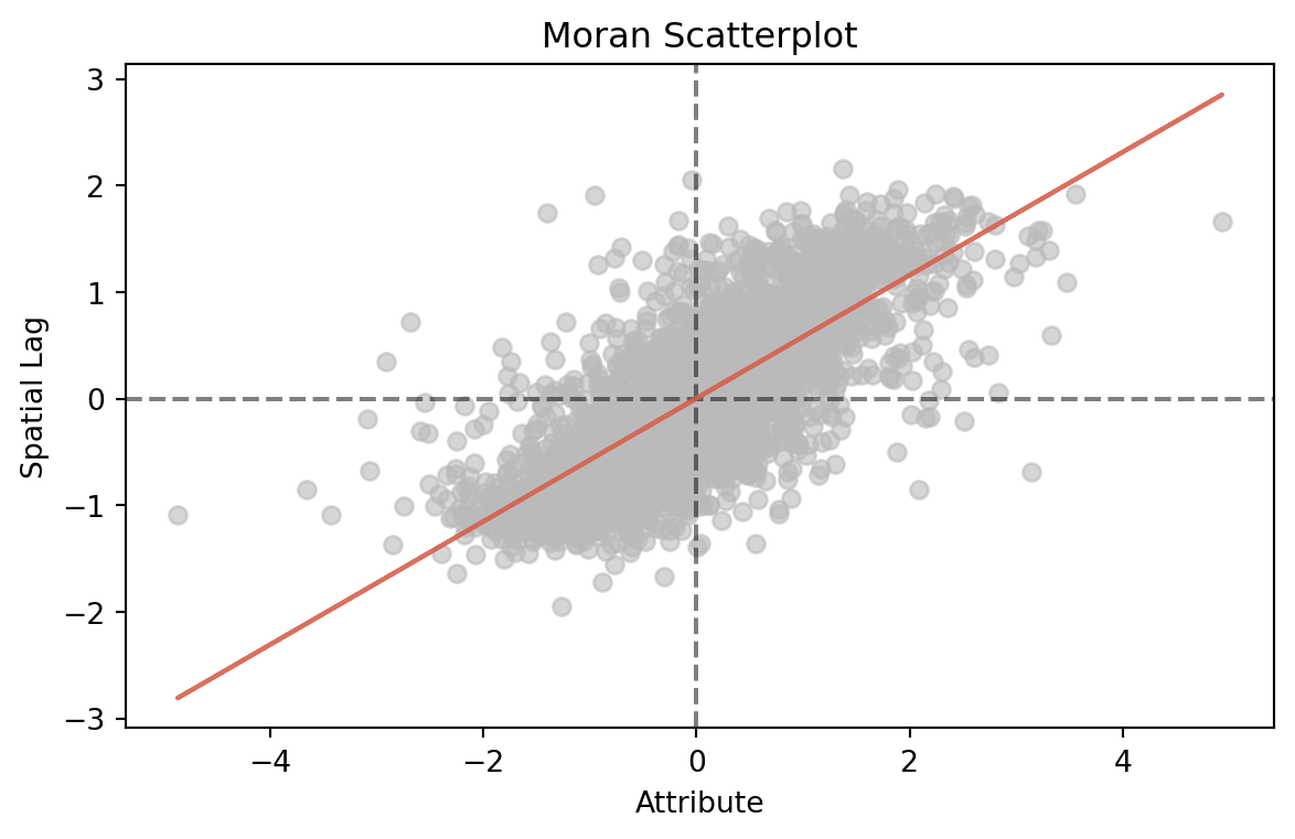

Moran’s I is significant and positive, indicating that this dataset has positive spatial autocorrelation. The Moran Scatterplot compares the (standardized) target variable to the weighted mean of nearby values (spatial lag). It confirms the I-value’s assessment of positive autocorrelation.

8.5.6 Kriging

Kriging is a nonparametric method of interpolation. Using the OrdinaryKriging class from PyKrige, we can estimate the mean of a parameter over the spatial plane.

from sklearn.model_selection import train_test_split
df_train, df_test = train_test_split(df, test_size=0.2, random_state=1234)

krige = pk.OrdinaryKriging(
    x=df_train["xcoord"],
    y=df_train["ycoord"],
    z=df_train["pct_voter"],
    coordinates_type="geographic" # use spherical coordinate math
)

# use trained model to estimate test data
df_test["krige_estimate"], _ = krige.execute(
    "points", df_test["xcoord"], df_test["ycoord"]
)

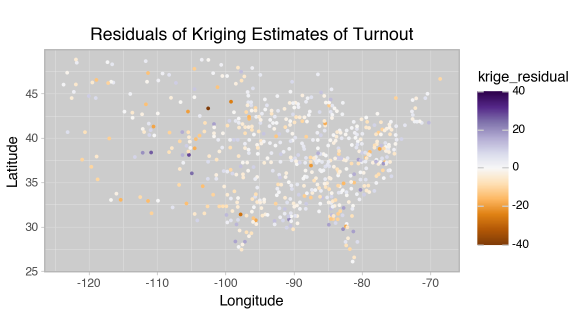
df_test["krige_residual"] = df_test["pct_voter"] - df_test["krige_estimate"]

With the model trained, we can check that it performs as expected on the test set.

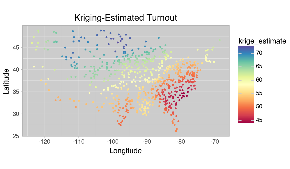
(ggplot(df_test, aes(x="xcoord", y="ycoord", color="krige_estimate"))
    + geom_point(size=0.6)
    + scale_color_continuous(cmap_name="Spectral")
    + coord_equal(ratio=1.3)
    + labs(
        title="Kriging-Estimated Turnout",
        x="Longitude",
        y="Latitude"
    )
    + theme_light()
    + theme(
        panel_background=element_rect(fill="#cccccc"),
        figure_size=(6, 3.5)
    )
)

(ggplot(df_test, aes(x="xcoord", y="ycoord", color="krige_residual"))
    + geom_point(size=0.6)
    + scale_color_continuous(
        cmap_name="PuOr",
        limits=(
            max(abs(df_test["krige_residual"])),
            -max(abs(df_test["krige_residual"]))
        )
    )
    + coord_equal(ratio=1.3)
    + labs(
        title="Residuals of Kriging Estimates of Turnout",
        x="Longitude",
        y="Latitude"
    )
    + theme_light()
    + theme(
        panel_background=element_rect(fill="#cccccc"),
        figure_size=(6, 3.5)
    )
)

(ggplot(df_test, aes(x="krige_residual", fill="krige_residual"))
    + geom_histogram(
        bins=20,
        fill="#99bbff",
        color="#000000"
    )
    + labs(
        title="Residuals of Kriging (No Regression)",
        x=f"Error (Percentage Points)"
    )
    + theme_light()
    + theme(
        figure_size=(6, 2.5)
    )
)

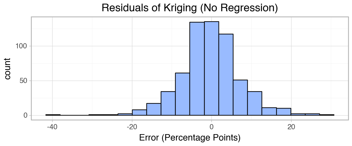
Variance seems to be higher in the west, where counties are farther apart, but the overall trend seems to be fit well. The errors seem approximately normal and the geographic patterns seen in the full dataset seem to be captured accurately by the method.

8.5.7 SEM Regression With Kriging

To compare performance with and without spatial components, we will use a basic linear regression model.

from sklearn.model_selection import train_test_split
from sklearn.linear_model import LinearRegression

X_train, X_test, Y_train, Y_test = train_test_split(
    X := df[["pop", "education", "houses", "income"]],
    Y := df["pct_voter"],
    test_size=0.2, random_state=1234
)

model_basic = LinearRegression().fit(X_train, Y_train)

print(f"Test R-squared: {model_basic.score(X_test, Y_test):.4f}")

(ggplot(
        pd.DataFrame({
            "Predicted Value" : model_basic.predict(X_test),
            "True Value" : Y_test,
            }), 
        aes(x="Predicted Value", y="True Value")
    )
    + geom_point(color="#00000088")
    + geom_abline(slope=1, intercept=0, color="red", linetype="dashed")
    + theme_light()
    + theme(figure_size=(4, 3))
)

Test R-squared: 0.4694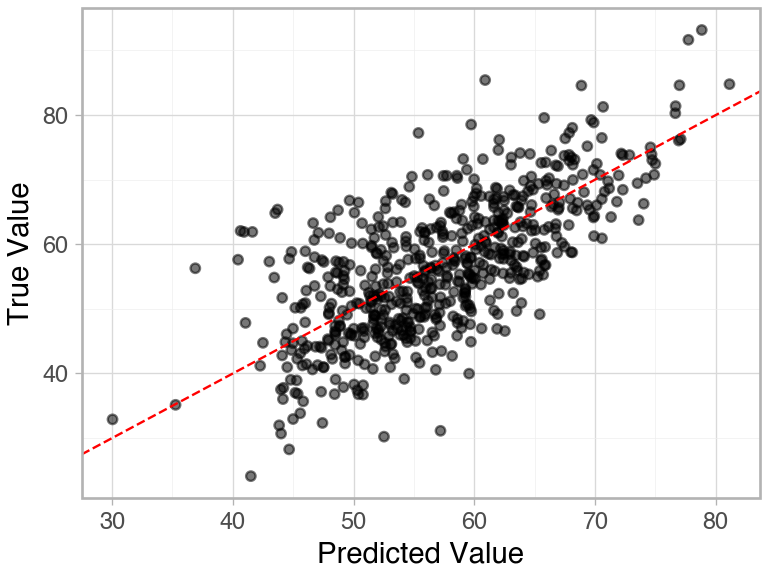

The data seem generally well fit, but there is a lot of unexplained variability. We can use Kriging on the residuals of the basic model to augment its performance.

df_train = df_train.reset_index()
df_test = df_test.reset_index()

p_train = df_train[["pop", "education", "houses", "income"]].to_numpy()
x_train = df_train[["xcoord", "ycoord"]].to_numpy()
y_train = df_train["pct_voter"].to_numpy()

p_test = df_test[["pop", "education", "houses", "income"]].to_numpy()
x_test = df_test[["xcoord", "ycoord"]].to_numpy()
y_test = df_test["pct_voter"].to_numpy()

from pykrige.rk import RegressionKriging

# any sklearn machine learning model can be used as the regression_model
model_rk = RegressionKriging(regression_model=LinearRegression())

# Note that predictors, points, and targets must be np arrays, not DataFrame
model_rk.fit(p_train, x_train, y_train)

Finished learning regression model
Finished kriging residuals

print(
    "R-squared (Regression + Kriging):",
    f"{model_rk.score(p_test, x_test, y_test):.4f}"
)
(ggplot(
        pd.DataFrame({
            "Predicted Value" : model_rk.predict(p_test, x_test),
            "True Value" : Y_test,
            }),
        aes(x="Predicted Value", y="True Value")
    )
    + geom_point(color="#00000088")
    + geom_abline(slope=1, intercept=0, color="red", linetype="dashed")
    + labs(title="Regression + Kriging")
    + theme_light()
    + theme(figure_size=(4, 3))
)

R-squared (Regression + Kriging): 0.6684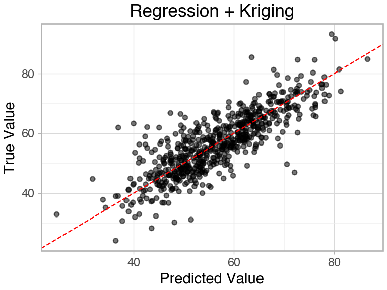

Spatially modeling the errors of the basic model allowed us to improve test set performance by over 40%.

8.5.8 Conclusions

PySAL offers strong tools for spatial data exploration and visualization. PyKrige lets you drop in spatial predictors or post-processing.

Spatial analysis is flexible. You can use spatial variables as part of the initial training (run OrdinaryKriging and use it as a predictor), or apply it at the end according to the SEM as demonstrated.

That being said, you have to validate the method. I had intended to demonstrate with the NYC Collision Data, but when I checked Moran’s I, the dataset had nonsignificant spatial autocorrelation. Crashes are largely independent events, so a spatial analysis would be fruitless. These tools are powerful, but can only be used in appropriate contexts.

8.5.9 Further Readings

ESRI’s explanation of spatial autoregression

The PySAL documentation

The PyKrige documentation

If you’re particularly interested in spatial problems and tools, GEOG 2500 (Introduction to Geographic Information Systems) is a good place to start learning about geographic methods.

The example image for Moran’s I and the Wikipedia article I got it from.

Nelder, J. A., & Wedderburn, R. W. M. (1972). Generalized linear models. Journal of the Royal Statistical Society Series A: Statistics in Society, 135(3), 370–384.

Pace, R. K., & Barry, R. (1997). Quick computation of regressions with a spatially autoregressive dependent variable. Geographical Analysis, 29(3), 232–247.