A Markov Chain is a mathematical system (stochastic model) that models a sequence of events where the probability of transitioning to the next state depends solely on the current state, not on previous history
Utilizes the memoryless property, meaning only the present state matters for predicting the future
9.1.2 Components of a Markov Chain
States: the possible situations/nodes the chain can be in at any given time
Can be represented by the state space (set of all possible states)
Transition Probabilities: measure the probabiliy of a stochastic system moving from one state to another within a specific timeframe or single step (represented by arrows)
Written mathematically as \[ p_{ij} = \Pr(X_{n+1} = j \mid X_n = i)\]
9.1.3 Example of Weather Markov Chain
Weather Markov Chain
9.1.4 A Transition Matrix
Definition: A square matrix that describes the probabilities of transitioning from one state to another
\(p_{ij}\) represents the probability of moving from state i to state j
All rows must sum to 1
We can create our transition matrix using a numpy array
import numpy as np# Create a 3x3 matrixmy_matrix = np.array([[0.7, 0.2, 0.1],[0.1, 0.6, 0.3],[0.2, 0.5, 0.3]])print(my_matrix)
[[0.7 0.2 0.1]
 [0.1 0.6 0.3]
 [0.2 0.5 0.3]]
9.1.5 Stationary Distributions
A stationary distribution of a Markov chain is a probability vector \[
\pi = (\pi_1, \pi_2, \dots, \pi_n)
\] that satisfies
\[
\pi P = \pi
\]
where P is the transition matrix. The values of \(\pi\) represent the long run probabilities of being in a specific state.
It also satisfies the normalization condition:
\[
\sum_{i=1}^{n} \pi_i = 1
\]
Stationary distributions are important because they describe the long-term behavior of a Markov chain regardless of the initial state.
9.1.7 Multistep Transition Probabilities in Markov Chains
Let P be the one-step transition matrix of a Markov chain.
The n-step transition probability from state i to state j is defined as
\[
p_{ij}^{(n)} = \Pr(X_n = j | X_0 = i).
\]
9.1.8 Matrix Interpretation
The matrix of \(n\)-step transition probabilities is given by
\[
P^{(n)} = P^n
\]
That is, the \(n\)-step transition matrix is simply the matrix \(P\) to the power of n ex. 2 step matrix is P times P Each row of \(P^n\) gives the distribution of the chain after \(n\) steps starting from a specific state.
9.1.9 Connection to Convergence
If the chain is irreducible and aperiodic (full loop), then
The rows of \(P^n\) converge to the stationary distribution.
The chain “forgets” its initial state.
9.1.10 Matrix Power Function
import numpy as npdef matrix_power(matrix, power):if power ==0:return np.identity(len(matrix))elif power ==1:return matrixelse:return np.dot(matrix, matrix_power(matrix, power -1))matrix_power(my_matrix, 1)
This is a good example of the memoryless property, the count two pitches ago doesn’t matter, only the count now
Transition probabilities were created using indexed pitching stats for each pitcher (normalized zone%, zoneswing%, oswing%, fair/foul%, compared to league average)
Based off these probabilities, we can find the stationary distribution that gives us expected K% and BB%
The observation depends only on the current hidden state:
\[
P(Y_t \mid X_t)
\]
For example:
If it is Rainy, cleaning or shopping probability might be high.
If it is Sunny, walking probability might be high.
9.1.12.6 Matrices
Remember we have a transition matrix describing how weather changes
Now we need a matrix to describe how the weather effects the activity, which is called an emission matrix
It defines the probability of a specific observable output symbol being generated from a particular hidden state
For N states and M observations, this is an N by M matrix
Rows sum to 1
9.1.12.7 Forward Algorithm
The forward algorithm is used in Hidden Markov Models (HMMs) to compute the probability of an observed sequence. Instead of listing every possible hidden state sequence (which grows exponentially), it uses dynamic programming to build the answer step by step.
At each time step, the algorithm keeps track of the probability of being in each hidden state, given all observations seen so far. It updates these probabilities by combining
the previous step’s probabilities
the transition probabilities between state
the likelihood of the current observation
By moving forward through time and updating these values recursively, the algorithm efficiently computes the total probability of the full observation sequence.
# 0 = Rainy, 1 = Sunny# 0 = walk, 1 = shop, 2 = cleanimport numpy as np# Initial probabilitiespi = np.array([0.6, 0.4])# Transition matrix AA = np.array([ [0.7, 0.3], # from Rainy [0.4, 0.6] # from Sunny])# Emission matrix BB = np.array([ [0.1, 0.4, 0.5], # Rainy emits walk, shop, clean [0.6, 0.3, 0.1] # Sunny emits walk, shop, clean])# Set our sequence of observationsobs = np.array([0, 1, 2]) # walk, shop, cleandef forward_np(obs, pi, A, B): T =len(obs) N =len(pi) alpha = np.zeros((T, N)) # creates empty matrix# Initialization. init state prob, multiplied by emission prob of first ob alpha[0] = pi * B[:, obs[0]]# Recursion. sums all ways to arrive in next weather state, multiplied by emission probfor t inrange(1, T): alpha[t] = (alpha[t-1] @ A) * B[:, obs[t]]# Termination. sums together all ways to observe the observation seq prob = np.sum(alpha[T-1])return alpha, probalpha, prob = forward_np(obs, pi, A, B)print("Forward matrix:\n", alpha)print("Total probability:", prob)
This matches the full sum over all 8 possible hidden state paths.
9.1.12.11 Viterbi Algorithm
The Viterbi Algorithm finds the most likely sequence of hidden states that could have generated a given observation sequence
How it works
Initialization: Initialize a probability matrix with the initial state probabilities multiplied by the emission probabilities.
Recursion: For each time step and state, calculate the highest probability of reaching that state from a previous state, keeping track of the best previous state using “backpointers”.
Termination: Find the maximum probability among the final states.
Path Backtracking: Follow the backpointers from the final, most likely state back to the beginning to reconstruct the optimal sequence.
def viterbi_np(obs, pi, A, B): T =len(obs) N =len(pi) delta = np.zeros((T, N)) # stores max prob of path ending in state j at time t psi = np.zeros((T, N), dtype=int) # stores index of prev state that gave max prob for j at t# Initialization delta[0] = pi * B[:, obs[0]] # initial prob times emission prob# Recursionfor t inrange(1, T): # loop over time steps for all statesfor j inrange(N): probs = delta[t-1] * A[:, j] # best prob of reaching i at t-1 times prob i to j psi[t, j] = np.argmax(probs) # store which prev state i gives max prob delta[t, j] = np.max(probs) * B[j, obs[t]] # max trans prob times emiss prob for current obs at j# Termination best_last_state = np.argmax(delta[T-1]) # chooses final state w highest pron best_prob = delta[T-1, best_last_state] # prob of best overall path# Backtracking best_path = np.zeros(T, dtype=int) # creates array to store best state sequence best_path[T-1] = best_last_state # set final statefor t inrange(T-2, -1, -1): # loop backwards best_path[t] = psi[t+1, best_path[t+1]] # follow backpointer to prev state that led to current bestreturn best_path, best_prob # return most likely seq and probabilitypath, prob = viterbi_np(obs, pi, A, B)print("Best path (state indices):", path)print("Probability of best path:", prob)
Best path (state indices): [1 0 0]
Probability of best path: 0.01344
9.1.12.12 Other Algorithms
9.1.12.12.1 Forward-Backward Algorithm
The Forward-Backward algorithm computes the probability of each hidden state at every time step given the full observation sequence.
It uses a forward pass to calculate the probability of observations up to each time step and a backward pass to calculate the probability
of the remaining observations. Multiplying these forward and backward probabilities and normalizing gives the posterior probability of being in each state at each time.
9.1.12.12.2 Baum-Welch Algorithm
The Baum-Welch algorithm is an Expectation-Maximization (EM) method used to learn the HMM parameters from observation sequences when hidden states are unknown.
It alternates between computing expected counts of state visits and transitions (E-step) and updating the initial, transition, and emission probabilities to maximize likelihood (M-step).
Repeating these steps iteratively improves the model to better fit the observed data.
9.1.12.13 Applications of HMMS
Financial Time Series Data
Algorithmic trading strategies
Credit risk modeling
Portfolio optimization
Interest rate modeling
Bioinformatics
Gene finding
DNA sequencing
Protein family modeling
9.1.12.14 Advantages and Limitations
9.1.12.14.1 Markov Chains
Advantages
Simple and easy to understand; only requires transition probabilities between states
Can be analyzed mathematically with well-established tools
Accurately models systems where only the present, not the past history, matters, which simplifies complex calculations
Can be applied to diverse fields, including marketing attribution (customer paths), finance (stock trends), gaming, and weather modeling
Limitations
Assumes the current state fully determines the next state (memoryless), which may be unrealistic
Transition probabilities must be known or estimated accurately, which can be hard for large state spaces
They predict the next state but do not explain why it happened (poor explanatory power)
They assume probabilities remain constant, failing to adapt to dynamic systems
9.1.12.14.2 Hidden Markov Models
Advantages
Can model sequences where the true states are hidden and only observations are seen
Captures uncertainty by using probabilities for transitions and emissions
Good at handling missing or incomplete data (power to infer states/observation)
Algorithms like the Forward-Backward algorithm and Viterbi algorithm provide polynomial-time solutions for training and decoding, ensuring fast inference
Limitation
Assumes Markov property and conditional independence of observations given states, which may not always hold
Performance heavily relies on the quality of initial parameter estimates (e.g., transition probabilities)
Hidden states may not have clear, real-world meaning, making results harder to interpret
With too many hidden states, HMMs can fit the training data very well but generalize poorly.
Hello! My name is Jonathan Trnka and this is my presentation on LLM Agents!
9.2.2 Objective
Quickly explain what an LLM is
Explain what makes an LLM-Agent different
Compare them
Explain my process
Use statistical tools to explain my Data
Conclusion
9.2.2.1 What exactly is an LLM Agent?
To put it simply, an LLM Agent is the next step in evolution of LLMs.
What is an LLM aka Large Language Model?
LLM chatbots are reactive conversational systems that receive user prompts, process them using pretrained knowledge, and generate text responses. Typical use cases include open-domain dialogue, customer support, and question answering. Despite being very powerful in their own way, they are still limited by outdated information and hallucinated responses.
What’s a hallucinated response you say?
A hallucinated response in regards to LLMs is when it creates incorrect, or fabricates content that believes is correct when it is not. For example, you could ask for a 5 step plan and it gives you 4 believe it to be correct. It’s all based on the prompt given to it by the user.
What does the ‘agent’ part mean?
The ‘agent’ part corresponds with the autonomous part of an LLM-Agent. This allows the LLM-Agent to resolve tasks on its own, without further input from a user. It can access APIs to access certain cotent, anything on the web, and solve errors it runs into.
What is RAG?
RAG, which stands for Retrieval Augmented Generation, is one approach to the limitations of standard LLMs. This is done by drawing real-time data from external sources such as APIs.
Limitations such as outdated information, single prompt answers, no recovery plans and so on.
9.2.3 LLM-Agent vs. Non‑LLM-Agent AI comparisons + examples
9.2.3.1 Table side-by-side Comparison
Aspect
LLM-Agent
Non‑LLM-Agent
Task Handling
Multi-step planning
Single-shot answer
Tool Use
Dynamic, context-driven
None
Accuracy
High on factual & numeric tasks
Variable; prone to errors
Adaptability
Adjusts plan mid-run
Fixed output
Error Recovery
Retries or switches tools
No recovery
Transparency
Shows steps & traces
Opaque
Latency
Slower
Fast
Cost
Higher
Low
Best For
Complex tasks
Simple tasks
9.2.3.2 Types of LLMs and LLM-Agents
Category
Model / System
Description
Agentic?
Standard LLM
GPT‑4o / GPT‑4 Turbo
General-purpose chat models; strong reasoning but no built‑in planning.
No
Standard LLM
Claude 3 Opus / Sonnet
High‑quality reasoning and writing; non‑agentic unless wrapped in a system.
No
Standard LLM
LLaMA‑3.1 / LLaMA‑3.2 / LLaMA‑3.3
Open models used in research; non‑agentic by default.
No
Standard LLM
DeepSeek‑V3
Efficient, high‑performance model; not agentic without a tool layer.
No
Standard LLM
Mixtral 8x7B / 8x22B
Sparse MoE models; strong performance but no autonomy.
No
LLM-Agent System
OpenAI o‑series with function calling
Uses planning + tool calls + multi‑step execution when orchestrated.
Yes
LLM-Agent System
Google Gemini 2.0 + Tools
Can plan, call APIs, and execute multi‑step tasks when tools are enabled.
Yes
LLM-Agent System
Groq LLaMA‑3.3 + my agent pipeline
Becomes agentic through my code of planning loops, tool calls, and error recovery.
Yes
LLM-Agent System
LangChain Agents
Framework that wraps any LLM with planning, tools, and autonomy.
Yes
LLM-Agent System
Microsoft Autogen Agents
Multi‑agent orchestration layer enabling planning and tool use.
Yes
LLM-Agent System
ReAct‑style LLM Agents
LLMs using reasoning + action loops to solve tasks step‑by‑step.
Yes
9.2.4 Specific Aims
My goal is to evaluate how effective a LLM-Agent system is compared to a baseline LLM. To do this, I will construct two models: an LLM-Agent capable of multi‑step planning, tool use, API integration, and limited error recovery, and a baseline LLM that processes only one prompt at a time without tool use or autonomous decision‑making. I will benchmark both systems on the same set of tasks and use linear regression techniques to analyze differences in performance, error rates, and execution time.
9.2.5 Data
9.2.5.1 My data will be from 1 non-api and 3 different API sources
Tavily (web search base)
OpenWeather
Calculator
Groq (the brain)
9.2.5.2 Main research question
“How well can an LLM-agent perform multi‑step tasks,self-recovery, accesseing API keys, replanning actions, compared to a baseline LLM that does not?”
9.2.5.3 Sub-research questions
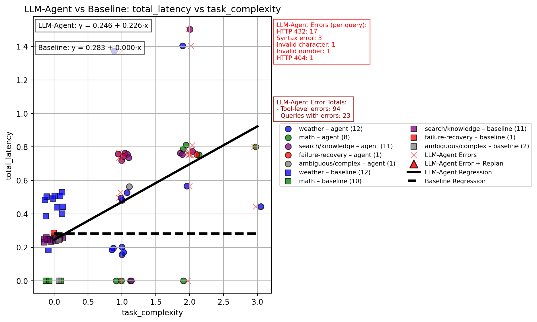
’Does the complexity(# of tool calls required to complete a task) of the task predict total_latency?
Y = total_latency
X = task complexity (# of tool calls required to complete a task)
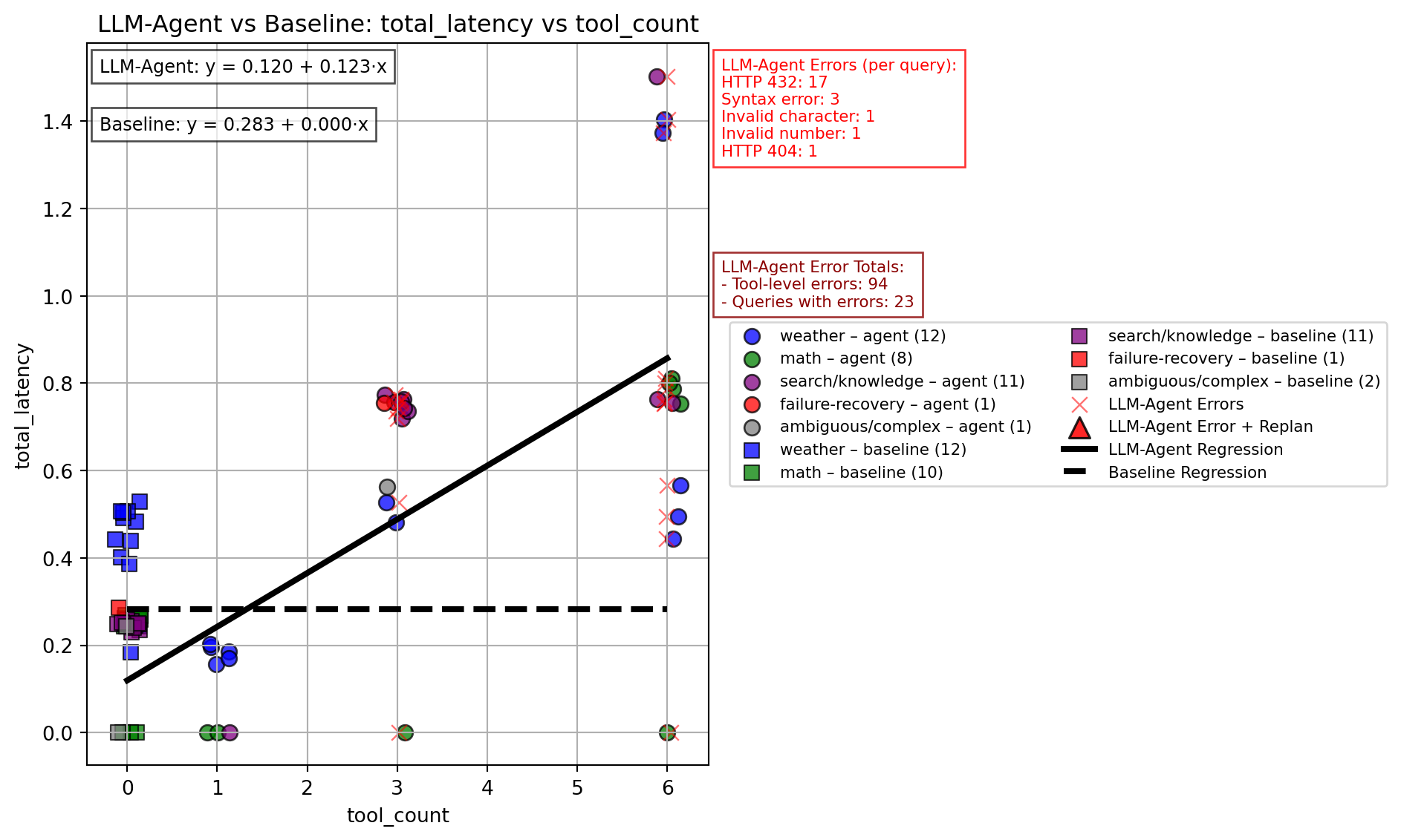
Does the number of tools(actual # of tool calls the agent executed) used predict total task latency?
Y = total_latency
X = task type
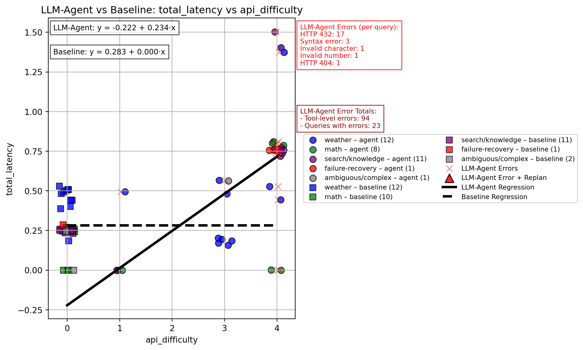
Does API difficulty predict total_latency?
Y = total_latency
X = API difficulty (numerical: calculator: 1, web-search:2, weather: 3)
9.2.6 Methods and Research Design
9.2.6.1 Experimental Framework
The study uses a between‑systems comparative design. Two AI systems are constructed: - LLM-Agent — a system capable of multi‑step planning, tool use, API calls, and limited error recovery. It can autonomously break down tasks, select tools, and retry operations when failures occur. - Baseline AI — a non‑agentic model restricted to single‑prompt, single‑response interactions. It cannot use tools, plan, or recover from errors. It behaves like a standard chat assistant. - Both systems are evaluated on identical tasks to isolate the effect of agentic capabilities.
9.2.6.2 Task Selection
Tasks are chosen to require reasoning, multi-step execution, or external information retrieval. Each task is designed so that: - The LLM-Agent system can leverage planning and tools. - The baseline system must attempt the same task without those capabilities. - Success, failure, and time-to-completion can be measured consistently.
9.2.6.3 Examples include
Multi-step problem solving (e.g., weather + calculation + summarization).
Error-prone tasks where retries matter (e.g., handling missing parameters).
9.2.6.4 Research Planning
Identify what my main research question would be and create my sub-research questions. All of which evaluate the performance of an LLM-Agent vs non-LLM-Agent (baseline)
Select and test my choosen variables.
task_complexity
api_difficulty
total_latency
tool_count
error count
9.2.6.5 Tool and Document Design
Chose tools that would be show multi-step agentic behavior. This would be weather retrieval, calculator functions, and web search.
Gather the required API keys and create a .ENV file. This would allow seamless access when executing code without hard-coding the credentials.
Create my ‘Agents_Multi_step’ python file. This holds all core functionality such as calling API keys, tool definitions, LLM-Agent and baseline LLM decision making, log functions, and more.
Create my ‘LLM_Agent_pipeline’ python file. This one holds code for running statiscal analysis, creating summary tables, the plots, the legends and more.
9.2.6.6 How it all comes together
Benchmark Queries (36 total) │ ▼
Run Agent + Baseline
Agent: multi-step, may call 0–many tools
Baseline: single LLM call │ ▼
Write Raw Logs
agent_runs.jsonl (one row per tool call)
baseline_runs.jsonl (one row per query) │ ▼
Load JSONL Logs inside the .qmd pipeline │ ▼
Clean + Aggregate
collapse retries
compute total latency
extract final answers
normalize errors
count tool usage
produce 1 row per query │ ▼
Export Clean Results to CSV summaries:
agentic_results.csv
baseline_results.csv │ ▼
Quarto Loads CSVs for regressions, plots, comparisons, and legends │ ▼
Generate Final PDF (plots, regressions, comparisons, summaries)
9.2.6.7 Before Diving in
6 questions for each type of query listed:
Math
weather
Web search
Multi Tool
Failure-recovery
Ambiguous/complex
Each question will have its own linear regression plot, a comparison table, an error summary, recovery actions used summary, and 2 legends on the linear regression plot. Legends for errors, the other for all queried data.
The LLM-Agent tries to “fix” the input and try again.
Next, it has the capability to switch tools.
Lastly, it will just use the baseline LLM. This option is used last.
9.2.6.8 Finally, Some Code
The original benchmark step wipes old .JSONL and .CSV files and reruns all 36 queries through the live Groq, OpenWeather, and Tavily APIs.
For this shared course repository, the render below is shown but not executed. The report uses the saved benchmark artifacts already included in the LLM-Agents/ folder so that it can be rendered without requiring API keys during normal course use.
import osdef reset_logs():"""Delete all JSONL and CSV log files so the next experiment starts clean.""" files_to_delete = ["agent_runs.jsonl","baseline_runs.jsonl","agent_runs.csv","baseline_runs.csv" ]for f in files_to_delete:if os.path.exists(f): os.remove(f)print(f"Deleted: {f}")else:print(f"Not found (skipped): {f}")# Start freshreset_logs()from Agents_Multi_step import run_full_benchmark_and_save_csvagentic_stats, baseline_stats = run_full_benchmark_and_save_csv()
Remark: To rerun this benchmark from scratch, set GROQ_API_KEY, OPENWEATHER_API_KEY, and TAVILY_API_KEY, then re-enable evaluation for the code chunk above.
9.2.6.9 Does the complexity (# of tool calls required to complete a task) predict total latency?
The comparison between LLM-Agents and a baseline LLM is clear. This data shows how multi-step reasoning, tool use, recovery actions, and API use can change how effective a LLM can be. You can cleary see how the LLM-Agent is able to handle errors, self recover, access API keys and do multi-step reasoning and use all of that to predict total latency. I hope I showed just how effective an LLM-Agent can be. Which one would you choose?
9.2.8 For those wanting more
https://www.vellum.ai/llm-leaderboard?utm_source=bing&utm_medium=organic (compares top LLM models and LLM-Agents)
Remember to use any AI tool responsibily. AI is a wonderful tool but can be very easy to rely on it! Do not blindly trust the AI! Use those critical problem solving skills on hand!
9.3 Animation
9.4 Data Science in Animation
9.4.1 Statistical Methods Behind Animation
This presentation was prepared by Ryan Jiang.
9.4.2 Introduction
9.4.2.1 Why Study Animation Through Statistics?
Modern animation is not simply digital drawing; it is the result of large-scale statistical estimation and computational modeling.
Behind every realistic animated film are mathematical models that simulate light transport, physical motion, and learned patterns from data.
Although audiences see characters and stories, what powers those visuals are integrals, optimization problems, and probabilistic algorithms.
9.4.3 Mathematical Foundation
9.4.3.1 The Rendering Equation
The rendering equation models how light leaves a surface by combining emitted light and reflected incoming light.
This equation conceptually says that outgoing light equals emitted light plus reflected incoming light.
The integral term means we are summing contributions from all possible incoming directions.
Because it is recursive and high-dimensional, it cannot be solved analytically for complex scenes since light bounces multiple times.
9.4.4 Computational Challenge
9.4.4.1 Why exact solutions are infeasible
Real scenes involve many light bounces, and each bounce adds more complexity because light transport is recursive.
Because of this recursion and the dimensionality of the integral, exact analytical solutions are impossible for complex environments.
Because of this, studios rarely compute exact solutions and instead rely on estimation.
9.4.5 Statistical Solution
9.4.5.1 Monte Carlo estimation in rendering
Monte Carlo methods approximate integrals by sampling random directions and averaging the results.
In rendering, this becomes an estimator of outgoing radiance based on randomly sampled light paths.
By the Law of Large Numbers, this estimator converges as sample size increases. However, finite sampling introduces variance — and in animation, that variance appears visually as noise..
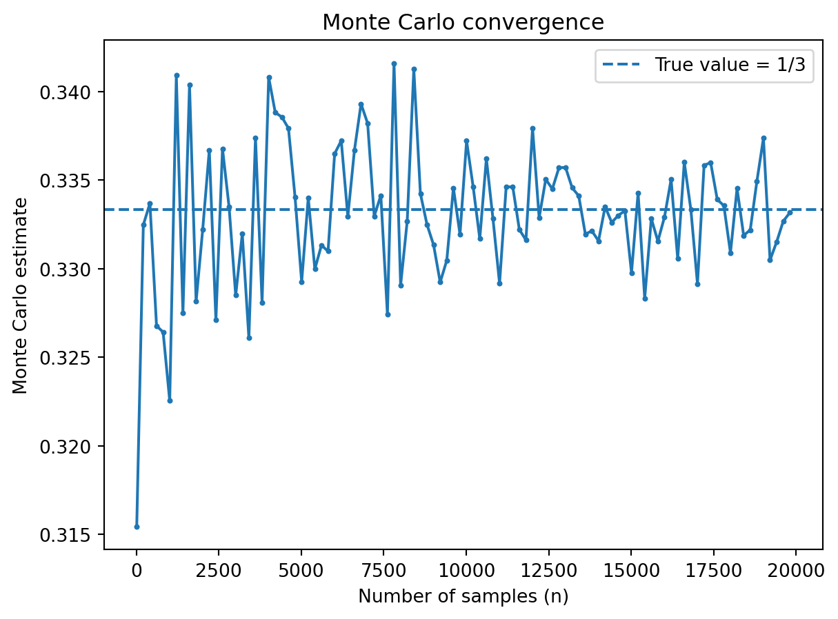
9.4.5.2 Monte Carlo convergence (integral estimation)
This demo estimates \(\int_0^1 x^2\,dx = 1/3\), illustrating how random sampling approximates an integral.
As shown, when the sample size is smalll, the estimate fluctuates but as the sample size increases, the estimate stabilizes around the true value.
This is exactly what happens in rendering: more samples per pixel reduce variability and produce smoother images.
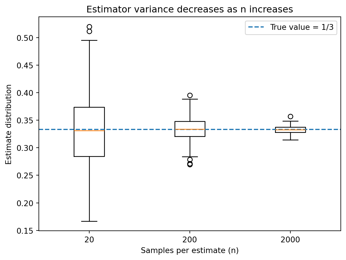
9.4.5.3 Variance reduction and noise analogy
This boxplot shows how estimator variability shrinks as sample size increases.
/var/folders/v8/ddhck0zx7h7c9kwqs57yzbvm0000gp/T/ipykernel_23342/830686255.py:18: MatplotlibDeprecationWarning:

The 'labels' parameter of boxplot() has been renamed 'tick_labels' since Matplotlib 3.9; support for the old name will be dropped in 3.11.
As shown on the plot, with only 20 samples, the estimates vary widely, but as samples increase, the distribution tightens around the true value of 1/3.
This shrinking spread represents decreasing variance, which in animation, corresponds to less visual noise.
9.4.6 Physics-Based Simulation
9.4.6.1 Modeling motion and natural phenomena
To animate cloth, hair, water, and smoke realistically, studios solve systems of differential equations numerically, like Newton’s second law:
[ F = m a ]
Acceleration is computed from forces such as gravity, tension, collision, and air resistance.
These continuous equations are approximated numerically using time-stepping algorithms.
If velocity changes over time, we approximate position updates using:
[ x_{t+1} = x_t + v_t t ]
Small time steps increase accuracy but increase computational cost.
Large time steps reduce cost but increase numerical error.
Numerical methods introduce discretization error, so step size and computational cost must be balanced.
Some systems incorporate randomness to simulate chaotic effects such as:
Smoke
Fire
Debris
Particle systems
Random forces are often drawn from probability distributions to mimic natural variation.
9.4.7 Optimization at Scale
9.4.7.1 Efficiency as a constrained problem
Rendering a single film may require millions of CPU hours.
Studios frame rendering as an optimization problem, minimizing variance subject to time and hardware constraints.
Techniques such as importance sampling and adaptive sampling allocate computational effort efficiently.
9.4.8 Machine Learning in Animation
9.4.8.1 Learning motion from data
Motion capture produces high-dimensional time series data that often contain noise and missing measurements.
Each frame of motion capture contains dozens of joint positions.
Over time, this produces high-dimensional time series data.
Noise, missing markers, and sensor errors require statistical smoothing.
Neural networks are trained to smooth motion and predict realistic joint trajectories.
Machine learning models predict future joint positions using regression:
[ = f_(x) ]
Where parameters ( ) are learned by minimizing a loss function.
Training involves minimizing a loss function through gradient-based optimization.
9.4.9 Generative AI
9.4.9.1 Diffusion models
Diffusion models generate images by learning to reverse a gradual noising process.
These systems approximate high-dimensional probability distributions over images.
They enable AI-assisted animation tools, frame interpolation, and visual synthesis.
9.4.10 Conclusion
9.4.10.1 Animation as Applied Data Science
Modern animation represents a collaboration between artists, engineers, statisticians, and data scientists.
What appears on screen is the result of probabilistic modeling, optimization, and computational simulation.
In this sense, digital storytelling is fundamentally powered by statistical methods.
9.4.11 Works Cited
Kajiya, J. (1986).The Rendering Equation. SIGGRAPH.
https://dl.acm.org/doi/10.1145/15922.15902
This foundational paper introduced the rendering equation, which models light transport in computer graphics.
Pharr, M., Jakob, W., & Humphreys, G. (2023).Physically Based Rendering: From Theory to Implementation. MIT Press.
https://pbr-book.org/
This book provides a comprehensive explanation of Monte Carlo rendering techniques used in modern animation.
Akenine-Möller, T., Haines, E., & Hoffman, N. (2018).Real-Time Rendering, Fourth Edition. AK Peters/CRC Press. https://www.realtimerendering.com/ This resource offers in-depth coverage of rendering algorithms, sampling techniques, and performance-oriented graphics methods relevant to animation.
Goodfellow, I., Bengio, Y., & Courville, A. (2016).Deep Learning. MIT Press.
https://www.deeplearningbook.org/
This foundational book explains neural networks and optimization methods used in motion modeling and AI-driven animation.
Rombach, R., et al. (2022).High-Resolution Image Synthesis with Latent Diffusion Models. CVPR.
https://arxiv.org/abs/2112.10752
This paper introduces diffusion-based generative models used in modern AI-assisted animation tools.