13  Advanced Topics

13.1 Filling Missing Data With Multiple Imputation

This section was prepared by Jacob Schlessel, a junior double majoring in Statistical Data Science and Economics.

13.1.1 Introduction

It is rare to work with a dataset that does not have missing values. This section will introduce multiple imputation as a method of filling these values and justify its use over other methods of imputation. The following topics will be covered:

1. Assessing Missingness

2. Benefits of Imputation

3. Limitations of Imputation

4. Methods of Single Imputation

5. Multiple Imputation

13.1.2 Assessing Missingness

Before filling in missing values, we must determine whether imputation makes sense given the context of the data. As a starting point, we can classify the missingness of the data into one of three different types. To illustrate the differences between these cases, we will use the following example:

A lab technician conducts a study on the relationship between age and blood pressure. Measurements are taken from a randomly selected group of 1000 volunteers, with all age groups being included in the study.

1. Missing completely at random (MCAR): the ideal case - missingness is independent of both observed and unobserved data
   • A lab technician accidentally forgets to record 10 patients’ blood pressure values because of a computer glitch
   • Missingness is random noise - estimates are not biased
2. Missing at random (MAR): the second best case - missingness depends only observed variables
   • Older patients are more likely to skip the blood pressure test because the cuff feels uncomfortable
   • Results are biased if you ignore the missing values
3. Missing not at random (MNAR): the missing values depend on the unobserved(missing) value itself
   • Patients with very high blood pressure intentionally refuse the test for fear of bad news
   • Imputation is not possible - requires advanced techniques like sensitivity analyses or pattern-mixture modes

Once we understand what type of missingness exists in the data, we have two options:

• Complete Case Analysis: Drop all rows with missing data and only include complete rows in analysis
• Imputation: Replace missing values with specific values, include filled values in analysis

13.1.2.1 Application in Python:

We wll use the airquality dataset from statsmodels as an example of working with missing data.

import statsmodels.api as sm
import pandas as pd

# Load the dataset
df = sm.datasets.get_rdataset("airquality").data

# Summarize missing data
missing_count = df.isna().sum()

missing_percent = (df.isna().mean() * 100).round(2)

missing_summary = pd.DataFrame({
    'Missing Count': missing_count,
    'Missing %': missing_percent
}).sort_values('Missing %', ascending=False)

print(missing_summary)

         Missing Count  Missing %
Ozone               37      24.18
Solar.R              7       4.58
Wind                 0       0.00
Temp                 0       0.00
Month                0       0.00
Day                  0       0.00

We cannot perform imputation if the data is MNAR. Therefore, to disprove that a dataset is MNAR, a good starting point is to look for evidence for MCAR or MAR, as a dataset cannot exhibit two different types of missingness. We do not actually need to know which of these two cases apply since imputation works with both, we just need to be able to confidently claim that the missing values are not associated with unobserved values and thus will not affect inference.

To find evidence of MCAR or MAR, we can use the following framework to analyze patterns of missingness:

1. Define the missingness target (the variable with missing values)

2. Perform statistical tests (t-tests for numeric, chi-squared tests for categorical) - note: this is not always conclusive

3. Find correlations between the target and other variables. If the correlation is above 0.2, this could be evidence of MAR and warrants further investigation

4. Use domain knowledge to perform in-depth analysis to rule out the possibility of MNAR missingness. Note: it is impossible to definitively prove or disprove MNAR based on the data because by definition, we do not have data to analyze.

Null hypothesis: The means for each variable are the same for the in the missing/nonmissing Ozone groups

Alternative hypothesis: The means for each variable are different for the in the missing/nonmissing Ozone groups

from scipy.stats import ttest_ind

# Create indicator: 1 if Ozone is missing, else 0
df['Ozone_missing'] = df['Ozone'].isna().astype(int)

for col in ['Solar.R', 'Wind', 'Temp']:
    group1 = df.loc[df['Ozone_missing'] == 0, col].dropna() 
    group2 = df.loc[df['Ozone_missing'] == 1, col].dropna()  
    stat, p = ttest_ind(group1, group2, equal_var=False)
    
    mean1 = group1.mean()
    mean2 = group2.mean()
    
    print(f"{col}:")
    print(f"  Mean (Ozone observed) = {mean1:.2f}")
    print(f"  Mean (Ozone missing)  = {mean2:.2f}")
    print(f"  p-value = {p:.4f}\n")

Solar.R:
  Mean (Ozone observed) = 184.80
  Mean (Ozone missing)  = 189.51
  p-value = 0.7846

Wind:
  Mean (Ozone observed) = 9.86
  Mean (Ozone missing)  = 10.26
  p-value = 0.5446

Temp:
  Mean (Ozone observed) = 77.87
  Mean (Ozone missing)  = 77.92
  p-value = 0.9787

The pvalues are all large, meaning the means are the same for each variable regardless of whether ozone is missing.

Since Month is a categorical variable, we can perform a chi-squared test to check if the number of missing values depend on the month:

Null hypothesis: The number of missing Ozone values does not depend on the month Alternative hypothesis: The number of missing Ozone values does depend on the month in some way

from scipy.stats import chi2_contingency

# Create contingency table: Month × Missingness
contingency = pd.crosstab(df["Month"], df["Ozone_missing"])
print("Contingency Table (Month vs. Ozone Missingness):\n")
print(contingency)

# Perform Chi-square test of independence
chi2, p, dof, expected = chi2_contingency(contingency)

print("\nChi-square test results:")
print(f"Chi-square statistic = {chi2:.3f}")
print(f"Degrees of freedom    = {dof}")
print(f"p-value               = {p:.4f}")

Contingency Table (Month vs. Ozone Missingness):

Ozone_missing   0   1
Month                
5              26   5
6               9  21
7              26   5
8              26   5
9              29   1

Chi-square test results:
Chi-square statistic = 44.751
Degrees of freedom    = 4
p-value               = 0.0000

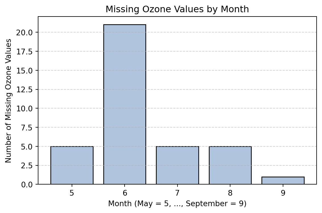
June has noticeably more missing Ozone values than the other months, so we confirm that this difference is statistically significant by observing a pvalue of 0. We can confirm this visually as well:

import matplotlib.pyplot as plt

# Plot number of missing ozone observations by month
missing_counts = (
    df[df["Ozone_missing"] == 1]["Month"]
    .value_counts()
    .sort_index()
)
missing_counts = (
    missing_counts.reindex([5, 6, 7, 8, 9], fill_value=0)
)
plt.figure(figsize=(6, 4))
plt.bar(
    missing_counts.index.astype(str),
    missing_counts.values,
    color="lightsteelblue",
    edgecolor="black"
)
plt.xlabel("Month (May = 5, ..., September = 9)")
plt.ylabel("Number of Missing Ozone Values")
plt.title("Missing Ozone Values by Month")
plt.grid(axis="y", linestyle="--", alpha=0.6)
plt.tight_layout()
plt.show()

Since the number of missing values of Ozone depends on observed data, we have determined that the missingness is MAR and we can continue with imputation.

We can follow the same process for analyzing the missingness of Solar.R.

df['Solar_missing'] = df['Solar.R'].isna().astype(int) #1 = Missing

#t test for numeric variables
for col in ['Ozone', 'Wind', 'Temp']:
    g1 = df.loc[df['Solar_missing']==0, col].dropna()
    g2 = df.loc[df['Solar_missing']==1, col].dropna()
    stat, p = ttest_ind(g1, g2, equal_var=False)
    print(col)
    print(f"Mean (Solar.R observed) = {g1.mean():.2f}")
    print(f"Mean: (Solar.R missing) = {g2.mean():.2f}")
    print(f"p-value = {p:.4f}\n")

#chi squared test for categorical variable (month)
cont = pd.crosstab(df['Month'], df['Solar_missing'])
chi2, p, dof, exp = chi2_contingency(cont)
print(f"Month vs Solar.R missingness: chi2={chi2:.2f}, p={p:.4f}")


# Bar chart of counts by month
missing_counts = (
    df[df["Solar_missing"] == 1]["Month"]
    .value_counts()
    .sort_index()
)
missing_counts = (
    missing_counts.reindex([5, 6, 7, 8, 9], fill_value=0)
)
plt.figure(figsize=(6, 4))
plt.bar(
    missing_counts.index.astype(str),
    missing_counts.values,
    color="lightsteelblue",
    edgecolor="black"
)
plt.xlabel("Month (May = 5, ..., September = 9)")
plt.ylabel("Number of Missing Solar.R Values")
plt.title("Missing Solar.R Values by Month")
plt.grid(axis="y", linestyle="--", alpha=0.6)
plt.tight_layout()
plt.show()

Ozone
Mean (Solar.R observed) = 42.10
Mean: (Solar.R missing) = 42.80
p-value = 0.9602

Wind
Mean (Solar.R observed) = 10.00
Mean: (Solar.R missing) = 9.00
p-value = 0.5343

Temp
Mean (Solar.R observed) = 78.12
Mean: (Solar.R missing) = 73.00
p-value = 0.3602

Month vs Solar.R missingness: chi2=11.14, p=0.0251

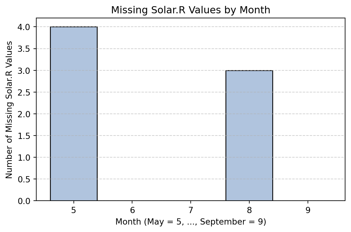
Similarly to Ozone, it appears that Solar.R is MAR since the missing values are related to the month during which the data was measured.

13.1.2.2 Important Notes

• Consider MNAR if domain knowledge suggests it

• Make sure to evaluate case-specific context to ensure imputation is appropriate. For example, using statistical imputation methods for the missing zip codes in the NYC Crash Data would not have made sense

• Proportion of missing data alone should not dictate whether imputation is used or not, need to use best judgement

13.1.3 Benefits of Imputation

Impututation replaces missing values with estimated ones to create a complete dataset. This process offers a number of benefits for modeling and analysis.

13.1.3.1 Preserving information

If we were to perform complete case analysis, we would lose the valuable information provided by the rows that may be missing values for one or two variables. By making an educated guess as to what the value would have been, we can

• Maintain real-world relationships observed among variables
• Preserve sample size to build models with higher precision
• Conduct robust analysis with messy data
• Enables use of statistical methods and machine learning models

13.1.3.2 Reducing bias

If the data are MAR, deletion will bias the results of any statistical modeling because the missing cases are systematically different from observed cases. To ensure that our data is representative of what we are studying, we can use fill missing values using estimates based on relationships that exist in our observed data. Imputation preserves covariances and joint distributions, so the result is lower bias in model coefficients.

Note: not all imputation methods have the same effect on reducing bias. Multiple imputation tends to minimize bias more than single imputation methods when data is MAR.

13.1.4 Limitations of Imputation

Imputation does not completely solve issues caused by missing data, it only alleviates them. It is important to note the following limitations of imputation to better understand when it is appropriate to use:

• Simple imputation methods distort distributions and can impact visualizations
• Need to acknowledge that imputing missing data adds some uncertainty
• Cannot correct cases where data are MNAR
• Can be very computationally expensive depending on method of imputation and complexity of data

13.1.5 Methods of Single Imputation

Single Imputation: Replacing each missing value with a single, fixed estimate

Types of single imputation:

1. Mean Imputation: Replacing missing values with the mean of the observed data
2. Median Imputation: Replacing missing values with the median of observed data
3. Mode Imputation: Replace missing values with the mode (for filling categorical data)
4. Hot-Deck Imputation: Replace a missing value with an observed value (a “donor” from a similar case)

For each method, we will fit a regression model with Temp as the response variable and Ozone, Solar.R, Wind, and Month as predictors. We will find the value of the coefficients and their standard errors after applying each method of imputation to compare the results.

13.1.5.1 Mean Imputation

We will replace all missing Ozone and Solar.R values with the respective means from the observed data:

# Encode Month as categorical and create dummy variables
df["Month"] = df["Month"].astype("category")
df= pd.get_dummies(df, columns=["Month"], drop_first=True)
df = df.astype(float)

# Assign predictor and response variables
x_var = [
    "Ozone", "Solar.R", "Wind", "Month_6", "Month_7", "Month_8", "Month_9"]

# Apply mean imputation and fit the regression model
df_mean = df.copy()

for col in ["Ozone", "Solar.R"]:
    df_mean[col] = df_mean[col].fillna(df_mean[col].mean())

y = df_mean["Temp"]
X = sm.add_constant(df_mean[x_var])
model = sm.OLS(y, X).fit()
results = pd.DataFrame({
    "Coefficient": model.params.round(4),
    "Std_Error": model.bse.round(4)
})

print(results)

         Coefficient  Std_Error
const        64.6504     2.3474
Ozone         0.0953     0.0207
Solar.R       0.0153     0.0054
Wind         -0.3807     0.1512
Month_6      11.7914     1.4211
Month_7      13.9666     1.4895
Month_8      14.5699     1.5075
Month_9      10.5281     1.4189

Benefits:

• Is sufficient if less than 5% of a particular variable is missing

Limitations:

• Underestimates variances -> does not add any spread to the data, standard errors and confidence intervals are too small
• Reduces natural variability
• Performs poorly if data is not MCAR
• Shrinks covariance -> coefficients are biased towards zero

13.1.5.2 Median Imputation

We can fit the same model, this time using median imputation:

df_median = df.copy()

# Apply median imputation and fit the model
for col in ["Ozone", "Solar.R"]:
    df_median[col] = df_median[col].fillna(df_median[col].median())

# 4) Define predictors and response
y = df_median["Temp"]
X = sm.add_constant(df_median[x_var])

# 5) Fit OLS regression
model = sm.OLS(y, X).fit()

# 6) Display coefficients and standard errors only
results = pd.DataFrame({
    "Coefficient": model.params.round(4),
    "Std_Error": model.bse.round(4)
})

print(results)

         Coefficient  Std_Error
const        64.6857     2.3324
Ozone         0.0965     0.0205
Solar.R       0.0150     0.0054
Wind         -0.3708     0.1509
Month_6      12.3827     1.4122
Month_7      14.0042     1.4848
Month_8      14.5675     1.5032
Month_9      10.4375     1.4178

Benefits:

• More robust to outliers than mean imputation

Limitations:

• Underestimates uncertainty
• Flattens the distribution by clustering values at the center

13.1.5.3 Hot-Deck Imputation

Hot-Deck imputation chooses the value from a similar observation in the current dataset to fill the missing values with. The “donor” can be chosen randomly or conditionally. Here. we will fill missing values with similar observations from the same month, since earlier we found that Month was related to the number of missing values of both Ozone and Solar.R.

import numpy as np

df_hot = df.copy()
rng = np.random.default_rng(42)

def hot_deck_impute(df, target_col, month_dummies):
    # Reconstruct Month number from dummies (5–9)
    df = df.copy()
    df["Month_num"] = 5
    for i, col in enumerate(month_dummies, start=6):
        df.loc[df[col] == 1, "Month_num"] = i

    # Impute missing values within same month
    for i in df[df[target_col].isna()].index:
        month = df.at[i, "Month_num"]
        donor_pool = df.loc[
            (df["Month_num"] == month) & (~df[target_col].isna()), target_col
        ]
        if donor_pool.empty:
            donor_pool = df.loc[~df[target_col].isna(), target_col]
        df.at[i, target_col] = rng.choice(donor_pool.values)
    return df.drop(columns="Month_num")

# Apply to missing targets and fit model
month_dummies = ["Month_6", "Month_7", "Month_8", "Month_9"]
for col in ["Ozone", "Solar.R"]:
    df_hot = hot_deck_impute(df_hot, col, month_dummies)

y = df_hot["Temp"]
X = sm.add_constant(df_hot[x_var])
model = sm.OLS(y, X).fit()
results = pd.DataFrame({
    "Coefficient": model.params.round(4),
    "Std_Error": model.bse.round(4)
})
print(results)

         Coefficient  Std_Error
const        66.0892     2.2664
Ozone         0.0929     0.0194
Solar.R       0.0128     0.0053
Wind         -0.4199     0.1475
Month_6      12.5071     1.4301
Month_7      13.6540     1.5196
Month_8      13.9432     1.5414
Month_9      10.0670     1.4339

Benefits:

• Preserves real data values -> borrowed from observed “donors”
• Retains covariance structure, keeping relationships realistic
• Works well in MAR cases

Limitations:

• Requires enough donor candidates to avoid highly biased results
• Can propagate outliers

13.1.6 Multiple Imputation

Instead of replacing the missing cases with a single guess, multiple imputation creates multiple guesses to incorporate some randomness that mimics real world uncertainty.

Multiple Imputation by Chained Equations (MICE): the most widely used implementation of multiple imputation

1. Define one target variable and start with simple guesses (mean/median imputation) for missing cases of the non-target variable

2. Fit a regression model for the target using all other variables as predictors

3. Impute the missing values of the target variable with the estimate generated by the regression

4. Repeat for all variables that have missing data, using your newly found imputations as training data

5. Repeat the process m times using different random draws to create m complete datasets. For each cycle, the coefficients for the regression models are sampled from the posterior distribution - essentially, the coefficients are randomly selected from their respective distributions of their plausible values

6. Fit the final model m times using the complete datasets and pool results using Rubin’s Rules to combine estimates and obtain valid inference

Rubin’s Rules: formulas for combining m regression results into one final set of estimates, correctly accounts for within-imputation variance and between-imputation variance.

Pooled Estimate (Mean of Coefficients)

\[ \bar{Q} = \frac{1}{m} \sum_{i=1}^{m} Q_i \]

• \(Q_i\): estimate (regression coefficient) from imputed dataset i
  
• \(\bar{Q}\): overall pooled estimate (average of all estimates)

---

Within-Imputation Variance: captures the uncertainty within each model

\[ \bar{U} = \frac{1}{m} \sum_{i=1}^{m} U_i \]

• \(U_i\): estimated variance from dataset i

---

Between-Imputation Variance: captures uncertainty across imputations

\[ B = \frac{1}{m - 1} \sum_{i=1}^{m} (Q_i - \bar{Q})^2 \]

---

Total Variance (Rubin’s Combined Uncertainty): combines both within- and
between-imputation uncertainty

\[ T = \bar{U} + \left(1 + \frac{1}{m}\right) B \]

---

Pooled Standard Error: the final standard error that accounts for both
model uncertainty and missing-data uncertainty, useful for inference

\[ SE(\bar{Q}) = \sqrt{T} \]

13.1.6.1 Summary Table

Symbol	Meaning	Interpretation
\(Q_i\)	Estimate from imputation i	e.g., regression coefficient
\(U_i\)	Variance from imputation i	\(SE^2\) from that model
\(\bar{Q}\)	Mean of all \(Q_i\)	Final pooled estimate
\(\bar{U}\)	Mean of all \(U_i\)	Within-imputation variance
\(B\)	Between-imputation variance	Variability across datasets
\(T\)	Total variance	Combined uncertainty
\(SE(\bar{Q})\)	Pooled standard error	\(\sqrt{T}\), used in inference

Scikit-learn’s IterativeImputer class simplifies this process.

Example using the airquality data:

from sklearn.experimental import enable_iterative_imputer 
from sklearn.impute import IterativeImputer

# Variables for imputation regression models
month_dummies = [c for c in df.columns if c.startswith("Month_")]
num_cols = ["Ozone", "Solar.R", "Wind", "Temp"] + month_dummies

# Variables for final regression omdel
x_vars = ["Ozone", "Solar.R", "Wind"] + month_dummies
y_var = "Temp"


# Number of imputations
M = 10

# To store results
coef_list, var_list = [], []

# Perform MICE 10 times
for m in range(M):
    imp = IterativeImputer(  # Performs chained equations 
        random_state=42 + m, # Different random seed every time
        sample_posterior=True, # Adds random noise
        max_iter=20 # Iterates thru models 20 times or until convergence
    )
    imputed = imp.fit_transform(df[num_cols])

    df_imp = df.copy()
    df_imp[num_cols] = imputed

    X = sm.add_constant(df_imp[x_vars])
    y = df_imp[y_var]
    model = sm.OLS(y, X).fit()

    coef_list.append(model.params)
    var_list.append(model.bse ** 2)

# Rubin’s Rules
coefs_df = pd.DataFrame(coef_list)
vars_df  = pd.DataFrame(var_list)

Q_bar = coefs_df.mean()
U_bar = vars_df.mean()
B     = coefs_df.var(ddof=1)
T_var = U_bar + (1 + 1/len(coef_list)) * B
SE    = np.sqrt(T_var)

pooled = pd.DataFrame({"MI Coefficient": Q_bar.round(4),
                       "MI Std_Error": SE.round(4)})
print(pooled)

         MI Coefficient  MI Std_Error
const           64.9348        2.2675
Ozone            0.0946        0.0211
Solar.R          0.0138        0.0054
Wind            -0.3213        0.1545
Month_6         11.2000        1.5068
Month_7         13.2032        1.5408
Month_8         13.8689        1.5867
Month_9          9.9381        1.4006

Notice that the standard errors for this method are larger than those from the single imputation methods. This is good -> we are correctly accounting for the increased uncertainty caused by missing data

13.1.7 Conclusion

• Imputation is an excellent tool for producing valid inference from datasets with missing data

• Before performing any type of imputation, you should get very familiar with your data and assess what type of missingness it exhibits

• The model results generated from using MICE have less bias but increased variance

13.1.8 Further Readings

• Overview of Multiple Imputation

• Multiple Imputation With Varying Proportions of Missing Data

• Workflow of Performing Imputation

13.2 Uniform Manifold Approximation and Projection

This section was prepared by Mark Zhang, an undergraduate at UCONN.

13.2.1 Introduction

Uniform Manifold Approximation and Projection (UMAP) (McInnes et al., 2018) is a powerful dimensionality reduction technique designed to visualize high-dimensional data in a low-dimensional space, such as 2D or 3D. Unlike linear methods like PCA, UMAP captures nonlinear structures, preserving local clusters while also maintaining the overall global patterns of the data. UMAP is utilized for clustering, data visualization, and data exploration.

13.2.2 Other Dimensionality Reduction Techniques

13.2.2.1 Principle Component Analysis (PCA)

• linear technique; projects data along directions of maximum variance.
• Preserves global structure fairly well but may lose local neighborhood. details.
• good for visualization of 2-3 PCs but cannot capture nonlinear structures.

13.2.2.2 t-distributed Stochastic Neighbor Embedding (t-SNE)

• finds distances between pairs of points, maps onto t dist.
• nonlinear technique; preserves local structure very well.
• can distort global relationships.
• often slower than UMAP for large datasets.

13.2.3 Algorithm Approach and Intuition

UMAP is a graph-based dimensionality reduction algorithm rooted in algebraic topology. It represents data as a fuzzy graph and finds a low-dimensional embedding that preserves both local neighborhoods and global structure.

13.2.3.1 Mathematical Foundations

1. Riemannian Manifold - UMAP assumes the data lies on a Riemannian manifold, a smoothly curved surface embedded in high-dimensional space.

2. Simplicial Sets - From algebraic topology, a simplex is the simplest geometric building block (a point, line, triangle, etc.), and a simplicial complex describes how these pieces connect to form a space. Geometrically a k-simplex is a very simple way to build a k-dimensional object.

13.2.3.2 Learning the manifold structure

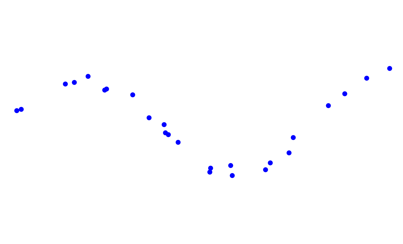
UMAP builds a graph as a discrete approximation of the manifold’s structure. To aid in visualizing the concepts, I will show how they apply to a noisy sin wave data set.

Test data set of a noisy sin wave

How do we represent this data as a manifold? UMAP uses the concept of simplicial sets and topology and adapts them to fuzzy simplicial sets and metric space.

13.2.3.2.1 Finding nearest neighbors

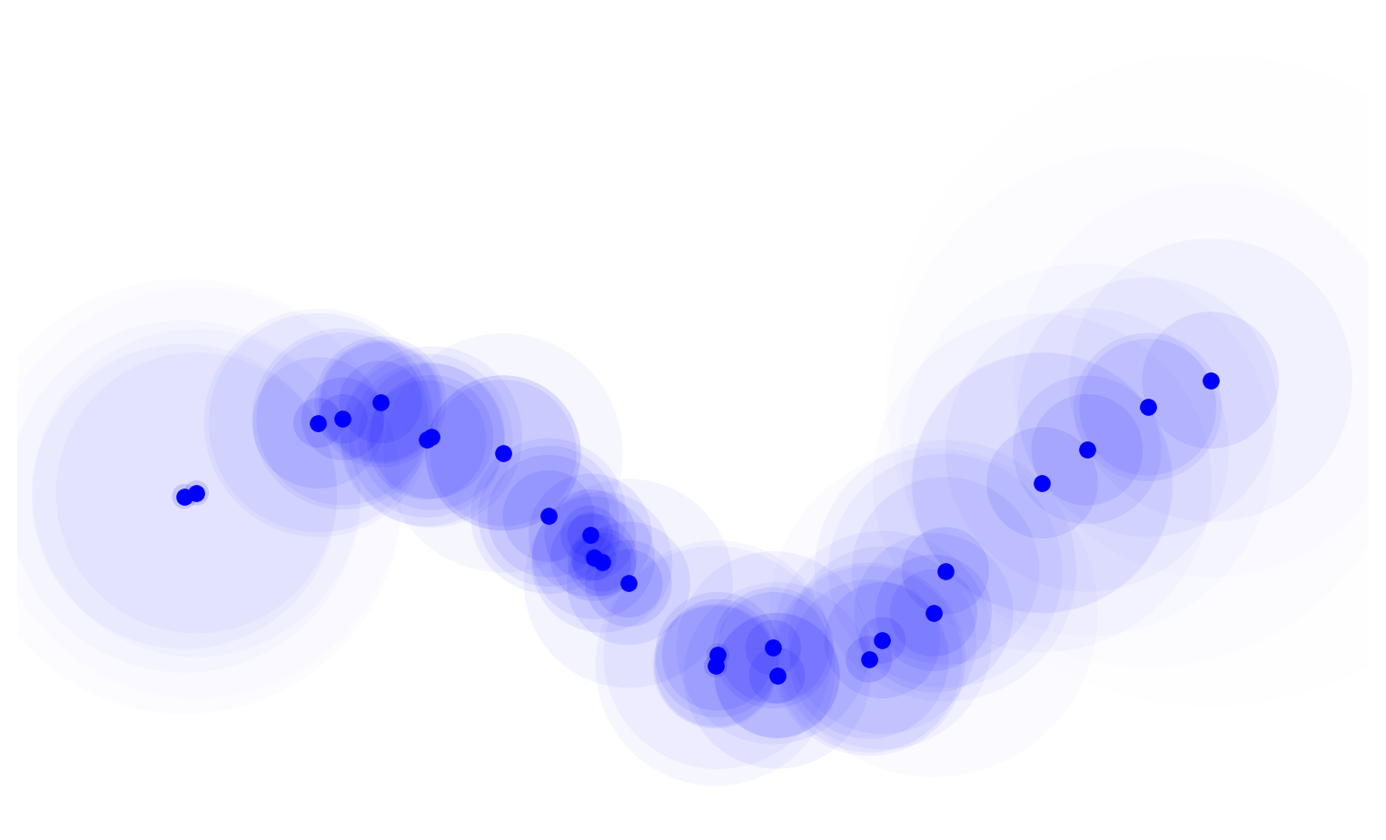
For each point we find the nearest neighbors. The nneighbors hyperparameter controls how local or global we want our structure to be. A large amount of neighbors represent the manifold more accurately as a whole and a smaller number would capture fine details of the structure.

Fuzzy circles to 4th nearest neighbor

13.2.3.2.2 Constructing a neighborhood graph

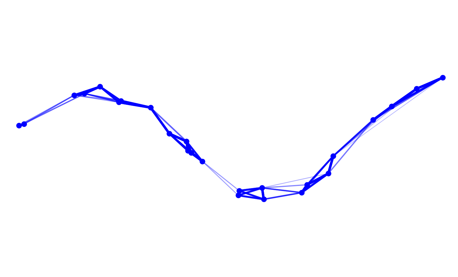
UMAP represents high-dimensional data as a fuzzy simplicial set, capturing the local connectivity of points. For each point, a fuzzy membership weight is assigned to its neighbors: \[ w_{ij} = \exp\Bigg(-\frac{d_{ij} - \rho_i}{\sigma_i}\Bigg), \]

where:

• \(d_{ij}\) is the distance between points \(i\) and \(j\),
• \(\rho_i\) is the distance to the closest neighbor of \(i\),
• \(\sigma_i\) is a local scaling factor.

In other words, each point adjusts its influence based on the local density of its neighborhood. Dense regions, where points are very close together, have smaller \(\sigma_i\), which reduces the weight of individual connections. Sparse regions, with points farther apart, have larger \(\sigma_i\). , increasing the weight of each connection.

Since \(w_{i \to j}\) and \(w_{j \to i}\) can differ, UMAP combines them using a probabilistic union:

\[ w_{ij}^{(final)} = w_{i \to j} + w_{j \to i} - w_{i \to j} \cdot w_{j \to i}. \]

This produces a symmetric weight between 0 and 1 that preserves local topology, balances contributions across dense and sparse regions, and yields a uniform manifold representation.

Fuzzy weighted graph with UMAP-style combined weights

13.2.3.3 Finding a low-dimensional representation

After building the fuzzy simplicial set (the weighted neighborhood graph), UMAP tries to embed the points in a low-dimensional space (e.g., 2D or 3D) while preserving the relationships encoded in the graph. This is done by optimizing a cost function.

13.2.3.3.1 Minimum Distance

The min_dist parameter controls how close points can be in the low-dimensional embedding:

• Small min_dist - points can be closer together, resulting in dense clusters that preserve fine local structure.
  
• Large min_dist - points are forced farther apart, producing spread-out clusters that highlight global relationships.

In other words, min_dist adjusts the tightness of clusters in the embedding without changing the underlying topology of the data.

13.2.3.3.2 Minimizing the cost function (Cross-Entropy)

After constructing the fuzzy simplicial set and initializing the low-dimensional embedding, UMAP positions the points by minimizing a cross-entropy-like cost function:

To compute the similarity between points in the low-dimensional embedding, UMAP defines a corresponding low-dimensional weight for each pair of points:

\[ w_{ij}^{(\text{low})} = \frac{1}{1 + a \|y_i - y_j\|^{2b}}, \]

where:

• \(\|y_i - y_j\|\) is the Euclidean distance between points \(y_i\) and \(y_j\) in the low-dimensional space (2D or 3D),
• \(a\) and \(b\) are hyperparameters that control the shape of the attraction/repulsion curve.

The cross-entropy cost function is then defined as: \[ C = \sum_{i \neq j} \Big[ w_{ij} \log \frac{1}{w_{ij}^{(\text{low})}} + (1 - w_{ij}) \log \frac{1}{1 - w_{ij}^{(\text{low})}} \Big], \] where: - \(w_{ij}\) = high-dimensional fuzzy weight between points \(i\) and \(j\), - \(w_{ij}^{(\text{low})}\) = corresponding low-dimensional embedding weight.

Intuition:

1. If two points are strongly connected in high dimensions (large \(w_{ij}\)), the embedding tries to place them close together.
   
2. If two points are weakly connected (small \(w_{ij}\)), the embedding tries to place them far apart.

UMAP uses stochastic gradient descent to minimize this cost function, adjusting the coordinates of points in low dimensions so that the embedding preserves both local neighborhoods and global manifold structure.

13.2.4 Practical Example: UMAP on 28x28 digit data

First, install the necessary dependency:

pip install umap-learn

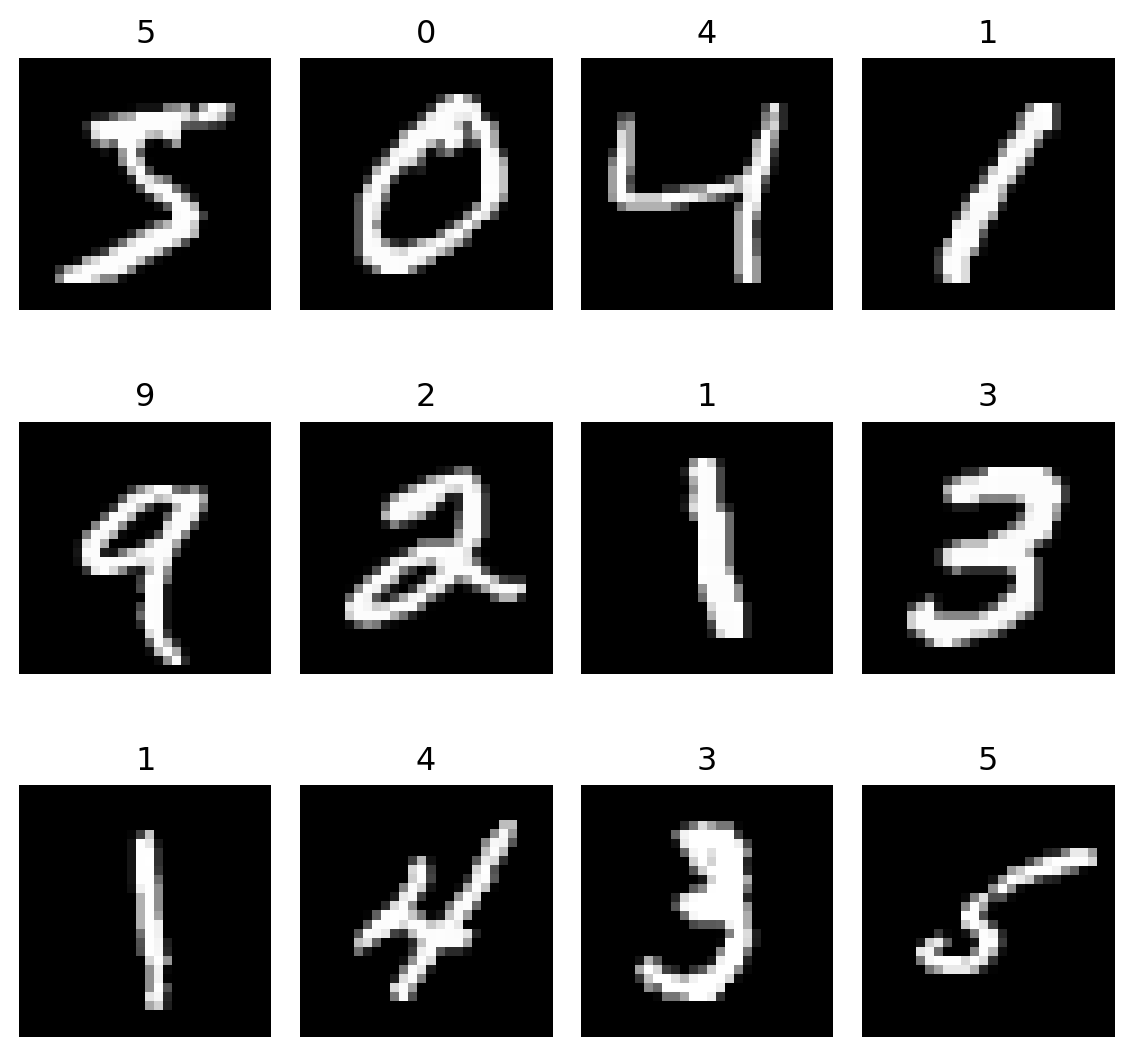
Before applying UMAP, let’s look at the raw data. The MNIST dataset from scikit-learn contains 70,000 images of handwritten digits, each represented as a 28×28 grayscale image (784 features per sample).

import matplotlib.pyplot as plt
import numpy as np
from sklearn.datasets import fetch_openml

# Load MNIST
mnist = fetch_openml("mnist_784", version=1, as_frame=False)
X = mnist.data[:2000]
y = mnist.target[:2000].astype(int)

# Reshape to 28×28 images
images = X.reshape(-1, 28, 28)

# Show first 12 digits in a 3×4 grid
fig, axes = plt.subplots(3, 4, figsize=(6, 6))
for i, ax in enumerate(axes.flat):
    ax.imshow(images[i], cmap='gray')
    ax.set_title(y[i])
    ax.axis('off')

plt.tight_layout()
plt.show()

Handwritten digit images (28×28) from MNIST dataset

We now project the 784-dimensional data into a 2D embedding using UMAP. The parameters below control the embedding:

• n_neighbors: how many nearby points are used to estimate local structure.

• min_dist: how tightly UMAP packs points in the low-dimensional space.

from umap.umap_ import UMAP
import matplotlib.pyplot as plt
import numpy as np
from sklearn.datasets import fetch_openml

# Load MNIST
mnist = fetch_openml("mnist_784", version=1, as_frame=False)
X = mnist.data[:2000]
y = mnist.target[:2000].astype(int)

# 2D UMAP projection
reducer = UMAP(
    n_components=2,
    n_neighbors=15,
    min_dist=0.1,
    random_state=42
)
X_umap = reducer.fit_transform(X)

# 2D scatter plot
plt.figure(figsize=(8, 6))
scatter = plt.scatter(
    X_umap[:, 0], X_umap[:, 1],
    c=y, cmap='tab10', s=5
)

plt.title("2D UMAP projection of MNIST (28×28)")
plt.xlabel("UMAP 1")
plt.ylabel("UMAP 2")
plt.colorbar(scatter, label='Digit')
plt.show()

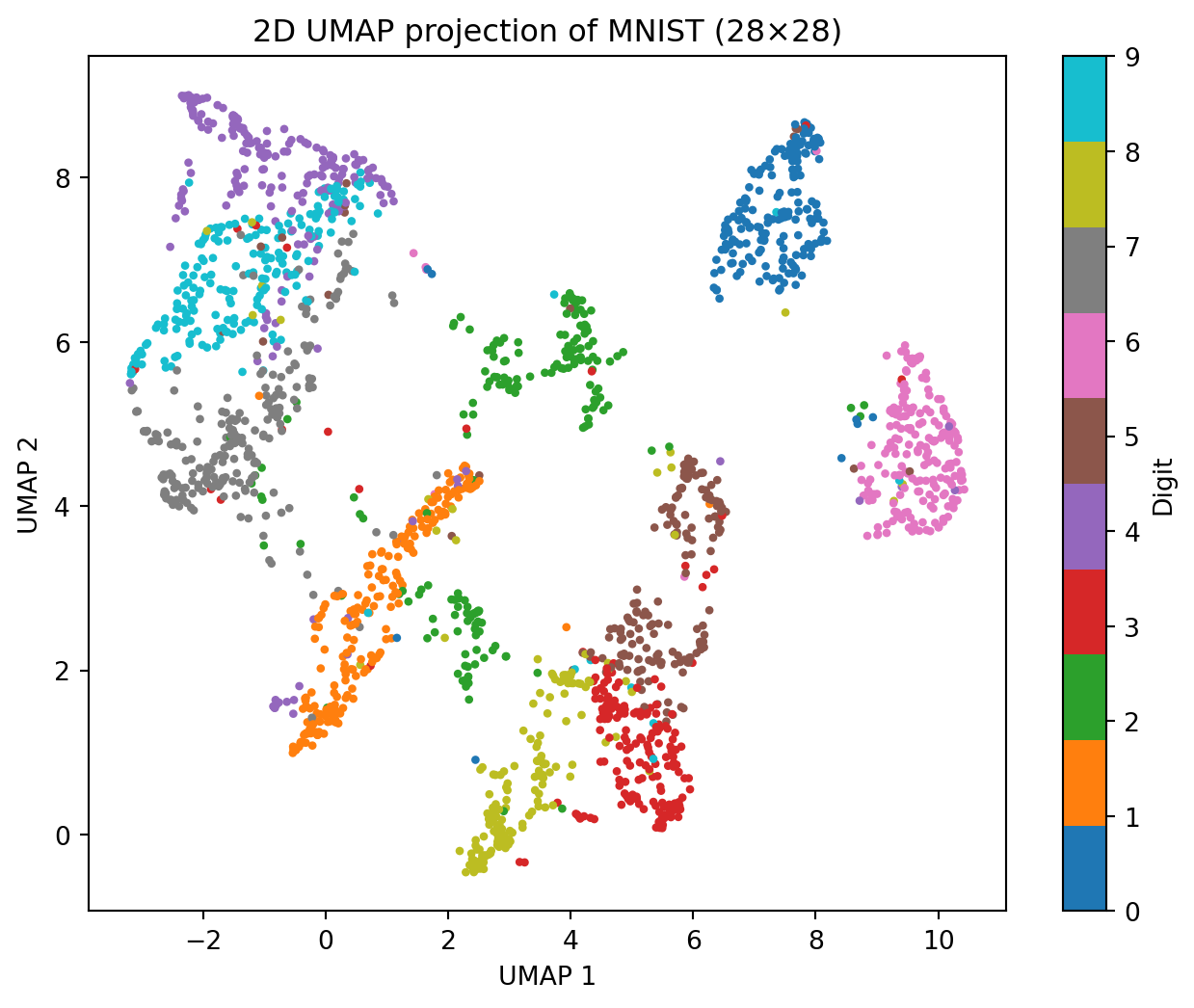
2D UMAP of MNIST dataset

In the 2D UMAP embedding of the digits dataset, each point represents a digit image, colored by its label. The plot shows that UMAP successfully captures the structure of high-dimensional data: points of the same digit cluster tightly, while visually similar digits appear near each other, preserving meaningful relationships.

• Same digits - form tight clusters, showing that UMAP preserves local neighborhood structure and keeps similar points together.
  
• Similar digits (e.g., 3 & 8) - positioned near each other, reflecting their visual similarity in shape and style.
  
• Different clusters - mostly separate, indicating clear class separation and that UMAP maintains distinctions between digit types.
  
• Global layout - reflects the relative positions of all clusters , preserving overall structure of the dataset.

Takeaway: UMAP reveals both local and global patterns, making high-dimensional data interpretable in 2D.

13.2.5 Conclusion

UMAP is a nonlinear dimensionality reduction technique that effectively captures both local and global structure in high-dimensional data. By constructing a fuzzy neighborhood graph and optimizing a low-dimensional embedding, it preserves cluster relationships, highlights visually similar points, and maintains overall manifold structure. This makes UMAP a powerful, interpretable tool for visualization and exploratory data analysis.

13.2.6 Further Readings

• UMAP Paper

13.3 How to call R from Python

This section was prepared by Wilson Tang, a undergraduate junior as of fall 2025 pursuing a single degree in statistical data science.

13.3.1 Motivations

R and Python are both languages we have been exposed to the most at UConn. I’ve had moments using one where I think about how the other might be useful, and so one might want to incorporate both languages. I want to show how we can properly incorporate R and Python together and when each language may be better.

Data science workflow:

Understanding the data science workflow will help us decide if we want to use R and Python together, or just individually.

• Identify problem
  
• Gather data
  
• Clean & preprocess data
  
• Data exploration
  
• Feature engineering / external data
• Statistical testing
  
• Modeling & machine learning
  
• Evaluation
  
• Visualization

13.3.2 Corresponding packages

For most tasks, we can find corresponding packages in both Python and R that can generally accomplish the same tasks. Of course, do mind exceptions can occur for very specific tasks and you should make decisions based on the scope of your work.

• Cleaning / Preprocessing Data
  • R: dplyr
  • Python: pandas
• Exploratory Data Analysis
  • R: built-in functions, dplyr, ggplot2
  • Python: pandas, matplotlib, seaborn, plotnine
• Feature Engineering
  • R: recipes (tidymodels), forcats, lubridate
  • Python: sklearn, pandas
• Evaluation
  • R: yardstick, caret
  • Python: sklearn, yellowbrick
• Visualization
  • R: ggplot2
  • Python: plotnine, matplotlib, seaborn

13.3.3 R / Python advantages

R:

• Statistical testing: t-test, ANOVA, chi-squared, Shapiro-wilk are common tests built into R. Durbin Test and a fisher’s test that can work for any r x c contingency table.
• Econometrics, time-series and biostatistics.

Python:

• Being able to handle bigger data
• Machine learning and AI
  • sklearn for machine learning
  • Tensor flow / Keras / Pytorch for deep learning
  • XGBoost / LightGBM / CatBoost for gradient boosting
  • Pipelines
    
• Versatile data handling
  • APIs - Better for large scale / complex integration (‘requests’, ‘httpx’, ‘aiohttp’)
  • Web Scraping - Better for large scale / dynamic web scraping (‘Beautiful’, ‘Scrapy’, ‘Selenium’)
  • Databases - SQL, NoSQL and big platforms
  • Cloud data - R has limited options for this and sometimes rely on Python libraries
  • Real-time data - R can’t really do this

13.3.4 Setup both R and Python

Make sure you have your own python:

Windows comes with python, however we want to install our own because it will prevent errors in the future steps. (Microsoft sucks)

Install python

Download R and Install R extension:

Install R

Find the Extensions tab on the left toolbar, search R language and install the R extension for VS code. And you can use Ctrl+Shift+P and type R: Create R terminal.

Calling R in Python:

We will use the package rpy2 to call R from Python, there are also other packages that can call R, check Additional resources.

Calling R from Python is a Python first method, and is generally recommended if the user is going to be using more python. However, one can also call Python from R as well. Check Additional resources for packages in R that allows us to call Python from R.

Reproducibility:

Since we are trying to use 2 languages at once, there will be packages from both R and Python. Of course, we would never want to compromise on reproducibility so what should we do? The best method would be to use Conda.

A single Conda environment can specify both versions of Python as well as R, while also allowing us to keep the packages of both in one place.

13.3.5 Example

Prerequisites:

In order to render these classnotes you will need to have a Python virtual environment with packages from requirements.txt and the package gamlss needs to be installed into your R global environment.

GAMLSS or Generalized Additive Models for Location, Scale, and Shape. It allows all parameters of the response distribution to depend on explanatory variables and thus each parameter can be modeled as a function of predictors. This model is useful when variability changes with predictors, skewness / kurtosis change with predictors.

Load Python libraries:

import pandas as pd
import seaborn as sns
import matplotlib.pyplot as plt

Load rpy2 to call R interface:

from rpy2 import robjects
from rpy2.robjects import pandas2ri, Formula
import rpy2.robjects.packages as rpackages
from rpy2.robjects.conversion import localconverter

Error importing in API mode: ImportError("dlopen(/Users/junyan/work/teaching/ids-f25/ids-f25/.ids-f25/lib/python3.13/site-packages/_rinterface_cffi_api.abi3.so, 0x0002): symbol not found in flat namespace '_R_BaseEnv'")
Trying to import in ABI mode.

Loading custom .RprofileLoading custom .Rprofile

Call gamlss from rpy2, rpy2 will look for the R global environment is the default location:

gamlss = rpackages.importr('gamlss')

Load in penguins from seaborn and prepare Data:

penguins = sns.load_dataset("penguins").dropna()

penguins = penguins.rename(columns={
    "body_mass_g": "mass",
    "bill_length_mm": "bill",
    "flipper_length_mm": "flipper"
})

penguins = penguins[["mass", "bill", "flipper", "species", "sex"]]

Send data frame from pandas to R and have it be converted to a R data frame using rpy2:

with localconverter(robjects.default_converter + pandas2ri.converter):
    r_df = robjects.conversion.py2rpy(penguins)

Here we are saying that mass depends on flipper, bill, species, sex and the variability of mass depends on flipper. Run gamlss from the R data frame to extract whatever we need from gamlss, in this case fitted \(\sigma\):

formula_mu = Formula("mass ~ flipper + bill + species + sex")
formula_sigma = Formula("~ flipper")

model = gamlss.gamlss(formula_mu, sigma_formula=formula_sigma,
                      data=r_df, family="NO")

fitted_sigma = robjects.r("fitted.values")(model, "sigma")

GAMLSS-RS iteration 1: Global Deviance = 4718.449 
GAMLSS-RS iteration 2: Global Deviance = 4718.415 
GAMLSS-RS iteration 3: Global Deviance = 4718.415 

Send fitted values or anything extracted from the previous part:

with localconverter(robjects.default_converter + pandas2ri.converter):
    penguins["fitted_sigma"] = robjects.conversion.rpy2py(fitted_sigma)

Use extracted values for anything of interest in Python, in this case let’s say for some reason we wanted to use matplotlib and seaborn to plot our fitted \(\sigma\):

plt.figure(figsize=(8,6))
sns.scatterplot(x="flipper", y="fitted_sigma", hue="species", data=penguins, 
                alpha=0.6)
sns.lineplot(x="flipper", y="fitted_sigma", hue="species", data=penguins, lw=2)
plt.title("GAMLSS: Predicted Variability vs Flipper Length")
plt.xlabel("Flipper Length (mm)")
plt.ylabel("Predicted Body Mass Variability (grams)")
plt.legend(title="Species")
plt.show()

We see here that as flipper length increases, predicted body mass variability tends to decrease.

13.3.6 Additional resources

• More packages to call R in Python and vice versa

• More about Python / R strengths and workflow with conda

13.4 Making a Personal Webpage on GitHub Pages

This guide will walk you through the process of creating your own personal website using GitHub Pages and Jekyll. We will cover setup to publishing and customizing the look of your site.

---

13.4.1 Introduction

My name is Jaden Mayer-Costa. I am a senior pursuing a Statistical Data Analysis degree with minors in both Economics and Music.

By the end of this guide, you should have the knowledge to create your own live site.

---

13.4.2 Why Use GitHub Pages?

GitHub Pages lets you host a website directly from your GitHub repository for free.
It’s ideal for portfolios, academic profiles, or blogs.

Key benefits:

• Free hosting with your own custom URL (username.github.io)
• Seamless integration with GitHub
• Built-in support for Jekyll, a static site generator
• No server or databases required

---

What is Jekyll?

Jekyll is a static site generator that can turn Markdown files into a lightweight website.

• Uses Markdown, templates, HTML, and CSS
• Generates static pages that load quickly
• Works easily with GitHub Pages
• Supports blogs, portfolios, and documentation sites

Why use it?

• You write simple Markdown → Jekyll reads and builds HTML → then push to GitHub Pages to host the site.

---

13.4.3 Setting Up Jekyll locally

First must install Ruby

Ruby is what Jekyll is written in and is necessary to download. You do not have to code in Ruby to use Jekyll, but it is what is running everything behind the scenes.

1. Visit RubyInstaller.org

2. Download the latest Ruby + Devkit version.

3. Run the installer and choose:

   • MSYS2 and MINGW development toolchain

4. After installation, open a new Command Prompt and check to ensure download was successful:

   ruby -v

   ---

Next, install Jekyll and Bundler from ruby

In terminal run

gem install jekyll bundler

What is a gem?: A gem is a Ruby package that basically represents a bunch of code or functionality that can be reused. Jekyll is an example of a gem.

Verify installation

jekyll -v

---

Finally, create a new Jekyll site

In terminal run

jekyll new personal-site

Jekyll will add all the necessary files for your site to run properly.

---

Run locally before pushing

Navigate to the personal-site file and preview your site locally by executing the code below.

jekyll new personal-site
cd personal-site
bundle exec jekyll serve

bundle exec is a command that runs a tool, in this case Jekyll, using the gems listed in the Gemfile.

After running and provided there are no errors, you Can then visit http://localhost:4000 to see your website.

What is bundler? bundler is a tool used to manage Ruby gems. It helps ensure your project uses the right versions of each gem that is listed in your Gemfile

What is a Gemfile? A Gemfile is simply a plain text file that lists all the Ruby gems your project needs in order to run. It is similar to what would be a “requirements.txt” file in Python. Essential to have for reproducibility.

Note: It is good practice to run your website locally before pushing to GitHub Pages to make sure your website will run before you make changes. Failure to check could result in a broken website.

13.4.4 Pushing to GitHub Pages

Create a GitHub repository to host files for website

• Go to GitHub
• Create a repository called: YOUR-USERNAME.github.io

---

Next, push your locally created site to GitHub

In terminal from the project folder run each of the following:

git init
git add .
git commit -m "GitHub Pages site made with Jekyll"
git branch -M test
git remote add origin https://github.com/username/username.github.io.git
git push -u origin main

Enable GitHub Pages on your repository

• Go to repository on GitHUb
• Go to Settings then click on pages
• Under “Source” click the test branch and / (root) folder
• Click Save - now website will be live at https://YOUR-USERNAME/github.io

13.4.5 Customizing Your Page

Now that your site is live, you can design and add personal touches. Jekyll gives control of layout, theme, colors, and structure while using simple files.

Standard layout

personal-website/
    _posts   # Blog posts
    _site   # Auto generated output
    .jekyll-cache   #Build cache
    _config.yml     # Main config file (controls theme, title, etc.)
    .gitignore      # Files git should ignore
    404.html    # Custom error page
    about.markdown      # About page
    Gemfile     # Lists Ruby dependencies
    Gemfile.lock    # Auto-generated dependency lock file
    index.markdown      # Homepage

---

Some different page types:

About Page:

• You can open about.markdown and edit this file to include a descriptive statement about yourself.

---
layout: page
title: About
permalink: /about/
---
Hello, my name is Jaden Mayer-Costa and I ...

Homepage:

• index.markdown is the landing page for your website. In other words this is the first thing that will be seen when visiting your site.
• Blog posts will appear here as well.

Blog Post:

• To add a new post navigate to your posts folder, add a markdown file, making sure to name it in YYYY-MM-DD-title.markdown format. Then in the yaml follow this template.

---
layout: post
title:  "title"
date:   YYYY-MM-DD HH-MM-SS
categories: jekyll update
---

• If you do not specify the date, Jekyll will not render the post.

---

Adding photos:

• Create an assets folder in your project root.
• Create a img folder in your assets folder and simply drop whatever pictures you want into your website there.
• To render a photo ensure it is in a jpg or png format.
• Here is the syntax to embed a picture:

![file_name]({{ '/assets/img/file_name' | relative_url }})

This tells Jekyll where to find your picture.

---

13.4.6 Themes

Jekyll has many different themes that allow you quickly restyle your site. By default Jekyll will use the minima theme, but if you go into the _config file, you can switch out to a different one, such as Cayman or Midnight. A more exhaustive list can be found on GitHub Pages

Minima is a good theme for beginners because it has everything we need to make a website without the need to create our own layouts, which can be time intensive. That’s why for the purposes of this tutorial, we will stick with minima.

Note: It is vital to pick a theme you like before building your website. Different themes have different layouts and dependencies, meaning you cannot easily change themes once a website is published.

13.4.7 Understanding Layouts in minima

Layouts are HTML templates that define how your pages and posts look. Having one is important to serve as a reusable frame or structure. Minima comes with four different layout options built in:

• default (Base HTML frame for all pages)
• home (lists posts on the homepage)
• page (Used for static pages like for an About or Project section)
• post (Individual blog posts)

Note: It is possible to override a layout by creating a custom _layouts folder where you can further customize your pages as desired. This is beyond the scope of this tutorial as it involves writing html code.

---

Adding New Tabs:

Say that we wanted to add a new tab to showcase the projects we have been working on in this class.

• We can create a projects.markdown file in our root folder.

• In the yaml add:

  ---
  layout: page
  title: Projects
  permalink: /projects/
  ---

• Add markdown content underneath.

13.4.8 Customize _config.yml

The _config file is where site settings are hosted. Things like title, URL, theme, and necessary plugins. Minima will automatically put a generic yaml to be filled out by the user. An example of a _config.yml setup is as follows:

# Preliminary information
title: "Personal Webpage on GitHub"
author: "Jaden Mayer-Costa"
email: "your@email.com"
description: "Data Analyst | Economist | Musician"
baseurl: "" # leave empty for main site
url: "https://jaden-m-c.github.io"

# Theme and plugins (pulling minima theme)
theme: minima
plugins:
  - jekyll-feed
  - jekyll-seo-tag

# Navigation links in the header
header_pages:
  - about.markdown
  - projects.markdown
  - blog.markdown

# Social media links
minima:
  social_links:
    github: jaden-m-c
    linkedin: your-linkedin

13.4.9 Changing colors and fonts

It is possible to make edits to a themes font and color without changing the entire theme through the use of a Cascading Style Sheet or CSS file.

• Create a file inside your assets folder called main.scss
• Import minima base styles into file:

---
---

@import "minima";

• Now can override original styles. Below example makes changes to the font weight, style, color, even footer background:

// Custom site styling
body {
  background-color: #fafafa;
  color: #222;
  font-family: "Inter", "Helvetica Neue", sans-serif;
}

a {
  color: #0057b7;
}

.site-title {
  font-weight: 700;
  font-size: 2rem;
  text-transform: uppercase;
}

footer {
  background: #111;
  color: white;
  padding: 1em 0;
}

13.4.10 Conclusion

You should know have the knowledge to set up a personal site on GitHub Pages using Jekyll. And any time you need to make an update, you can follow the workflow of makings edits and rendering locally before pushing to Pages. In this way, your page can evolve alongside your career. This overview is the basic setup to get a page, but there are truly so many ways to customize and edit your page to better reflect your personality and style.

13.4.11 Further Reading

• Using Jekyll in GitHub Pages
• Using themes from Jekyll
• GitHub Pages breakdown
• Resource to find themes for webpage

13.5 Web Scraping

This section was prepared by Sahil Patel, an undergraduate junior majoring in Computer Science, Statistical Data Science, and Economics.

13.5.1 An Introduction to Web Scraping

13.5.1.1 What is Web Scraping

Web scraping is a way to automatically gather information from websites. Instead of spending hours copying and pasting data, you can use scripts to collect large amounts of structured information quickly and consistently. Once you have the data, it can be analyzed, stored, or used for research and decision making.

Web scraping is particularly useful because most web data is created for humans to read, not for machines to process. By scraping, we can turn that information into a format that computers can work with, allowing us to explore trends, track changes, or gain insights that would be really hard to collect manually.

13.5.1.2 Use Cases of Web Scraping

Here are some of the use cases of web scarping:

• Market Analysis
  • Companies use web scraping to track products, prices, and customer reviews, helping them understand market trends and stay competitive.
• Finance and Investment
  • Analysts gather stock prices, financial news, and reports to make informed investment decisions or to analyze market sentiment.
• Academic Research
  • Researchers collect articles, datasets, and public records to support studies and uncover insights across a variety of fields.
• Social Media and Marketing
  • Marketers and analysts monitor trends, hashtags, and audience engagement to understand consumer behavior and improve campaigns.

13.5.1.3 Static versus Dynamic Web Pages

Before scraping, it is important to understand the kind of web pages you are working with:

• Static Web Pages
  • The content is already in the HTML when the page loads. Everything you need is there, so extracting it is relatively straightforward.
• Dynamic Web Pages
  • The content is generated by JavaScript or updated after the page loads. Fetching the HTML alone may not give you what you want. You may need to interact with the page to see the full content.

13.5.1.4 Legal and Ethical Considerations

Even though web scraping can be extremely powerful, it comes with important responsibilities and best practices that should not be ignored.

• Respect robots.txt: Before scraping a site, check its robots.txt file to understand which pages or sections the website owner allows you to access, and make sure to follow these guidelines.

• Avoid overloading servers: Sending too many requests too quickly can strain a website’s server. Introduce pauses between requests, use random delays, and keep your scraping activity at a reasonable pace to avoid causing problems for the website.

• Do not collect sensitive information: Avoid scraping personal, confidential, or protected information unless you have explicit permission to do so, as this could violate privacy laws or ethical standards.

• Check copyright and licensing: Just because you can access the data does not mean you have the right to use or redistribute it freely. Always review the site’s terms of use and any applicable copyright rules.

• Be transparent: When using scraped data in reports, analyses, or projects, clearly cite your sources and acknowledge where the information came from. Transparency helps maintain credibility and respect for the original content creators.

13.5.2 Basics of Web Requests

Before you can extract any data from a website, you need to first fetch the content of the page. In Python, this is typically done using the requests library, which allows you to send HTTP requests and receive responses. Understanding how these requests work is key to effective web scraping.

If you haven’t done so already, you will need install requests to your terminal.

pip install requests

13.5.2.1 HTML Basics

To scrape web pages effectively, it is important to understand the basic structure of HTML, which is the language used to create web pages. Web pages are made up of elements enclosed in tags. Some common tags include:

• <body>: this tag identifies the main body of the website, which contains the content that is visible to users.

• <table>: This tag identifies a table element, which is used to organize data in rows and columns.

• <tbody>: This tag identifies the body of the table, which contains all the rows of the table.

• <tr>: This tag identifies a table row, which contains individual cells (<td>) with data.

13.5.2.2 Response Status Codes

Every HTTP request returns a status code that indicates whether it was successful.

• 200 means the request was successful, and the server returned the requested content.
• 404 means the page was not found, which usually indicates the URL is incorrect.
• 403 means access is forbidden, which often happens when a server blocks automated requests.
• 500 indicates a server error on the website.

Checking these codes allows you to handle errors gracefully and avoid scraping pages that are unavailable or blocked.

13.5.2.3 HTTP Methods

The two most common HTTP methods used in web scraping are GET and POST.

• GET requests are used to retrieve data from a web server. This is the method you will use most often because you are usually trying to download the content of a page.
• POST requests are used to send data to a server, often when submitting forms or interacting with a website. Some websites require POST requests to access certain content or search results.

13.5.2.4 Using Headers and User-Agent Strings

Web servers sometimes treat automated requests differently from requests made by real browsers. By adding headers, you can make your requests look more like they are coming from a normal user.

A common header to include is the User-Agent, which identifies the browser and device making the request. Here is an example of what a header can look like:

import requests

url = 'https://uconn.edu'
headers = {
    'User-Agent': 'Mozilla/5.0 (Windows NT 10.0; Win64; x64) AppleWebKit/537.36 '
                  '(KHTML, like Gecko) Chrome/117.0.0.0 Safari/537.36'
}

response = requests.get(url, headers=headers)
print(response.status_code)  # prints the HTTP status code
print(response.text[:500])   # prints the first 500 characters of the HTML

200
<!DOCTYPE html>
<html lang="en-US" class="no-js">
<head>
    <meta charset="UTF-8">
    <meta name="viewport" content="width=device-width, initial-scale=1.0">
    <meta http-equiv="X-UA-Compatible" content="ie=edge">
    <link rel="profile" href="http://gmpg.org/xfn/11" />
    <link rel="pingback" href="https://uconn.edu/xmlrpc.php" />
    <title>University of Connecticut</title>
        <script type="application/ld+json">
        {
            "@context": "http://schema.org",
            "@type

13.5.3 An Introduction to BeautifulSoup

BeautifulSoup is one of the most popular Python libraries for web scraping. It helps you collect and organize information from web pages written in HTML or XML. When you look at a web page’s source code, it often looks like a confusing block of text. BeautifulSoup turns that chaos into a clean, organized structure that you can easily search and navigate. It is a reliable tool for collecting data from static websites such as news articles, course lists, or research archives.

13.5.3.1 Installing and Importing BeautifulSoup

To use BeautifulSoup, you first need to install it.

pip install beautifulsoup4

Once installed, import it into your Python script:

from bs4 import BeautifulSoup

BeautifulSoup works well alongside the requests library, creating a simple and efficient way to download and process web pages.

13.5.3.2 Loading HTML into BeautifulSoup

Once you have downloaded the HTML content of a web page, the next step is to load it into BeautifulSoup.

url = "https://decisiondrivers.com/nyc/zip-code/"
headers = {
    "User-Agent": "Mozilla/5.0 (Macintosh; Intel Mac OS X 10_15_7) AppleWebKit/537.36 "
                  "(KHTML, like Gecko) Chrome/117.0.0.0 Safari/537.36"
}

response = requests.get(url, headers=headers)
print("Status code:", response.status_code)

soup = BeautifulSoup(response.text, "html.parser")

Status code: 200

The requests.get() function fetches the page, and BeautifulSoup() parses it into a structure that can be easily searched. The "html.parser" argument tells BeautifulSoup how to interpret the HTML. The resulting soup object becomes your workspace for exploring and extracting information. You can now search for tags like <table>, <tr>, or <td> to extract the data you need.

Since the status code prints 200, that means the request worked successfully and the page’s content is ready to scrape.

13.5.3.3 Navigating and Searching the Parse Tree

BeautifulSoup organizes the HTML into a tree like structure that you can move through. Each tag, paragraph, or link becomes something you can directly access.

The most common ways to search are find(), find_all(), and select().

• find() – finds the first instance of a tag
• find_all() – finds all instances of a tag
• select() – finds elements using CSS selectors

# Find the first heading on the page
heading = soup.find('h1')

# Find all links on the page
links = soup.find_all('a')

# Use a CSS selector to find specific items
nav_links = soup.select('nav a')

13.5.3.4 Extracting Data

Before writing any scraping code, it’s helpful to understand where the data actually sits within the webpage. You can right-click anywhere on the site and choose Inspect to open your browser’s developer tools. This reveals the HTML structure of the page, where information is organized using tags such as <table>, <tr>, and <td>. These tags define how the data is arranged, helping you identify exactly which elements you’ll need to target with BeautifulSoup.

For example, on the [Decision Drivers NYC ZIP Codes] (https://decisiondrivers.com/nyc/zip-code/) page, the ZIP code information is not stored inside a table but listed under each borough heading. Every borough name appears as a heading tag, such as <h2>, followed by a list of ZIP codes written in plain text or inside <ul> and <li> tags. Instead of looping through table rows, you can search for each heading, record the borough name, and then capture the ZIP codes that appear beneath it. This structure works well with BeautifulSoup because it allows you to identify the borough from the heading and pair it with its corresponding ZIP codes by reading the text that follows.

import pandas as pd

boroughs = []
zips = []

# Split the entire text into lines, then look for boroughs and ZIPs
lines = soup.get_text("\n", strip=True).splitlines()
current_borough = None

for line in lines:
    text = line.strip()
    # If the line is a borough name, update the current borough
    if text.upper() in ["MANHATTAN", "BROOKLYN", "QUEENS", "BRONX", 
    "STATEN ISLAND"]:
        current_borough = text.title()
        continue

    # If the line is a 5-digit number, it’s a ZIP code
    if current_borough and text.isdigit() and len(text) == 5:
        boroughs.append(current_borough)
        zips.append(text)

# Create a clean DataFrame
df = pd.DataFrame({"Borough": boroughs, "ZIP": zips})
df = df.drop_duplicates().sort_values(["Borough", "ZIP"]).reset_index(drop=True)

# Display the first few rows
print(df.head(10))
print("\nTotal ZIP codes found:", len(df))

  Borough    ZIP
0   Bronx  10451
1   Bronx  10452
2   Bronx  10453
3   Bronx  10454
4   Bronx  10455
5   Bronx  10456
6   Bronx  10457
7   Bronx  10458
8   Bronx  10459
9   Bronx  10460

Total ZIP codes found: 179

13.5.3.5 Extended Example

This is an example that will be useful for our midterm assignment. Here, we scrape the addresses of all the precincts in NYC.

url = "https://www.nyc.gov/site/nypd/bureaus/patrol/precincts-landing.page"
headers = {
    "User-Agent": "Mozilla/5.0 (Macintosh; Intel Mac OS X 10_15_7) AppleWebKit/537.36 "
                  "(KHTML, like Gecko) Chrome/117.0.0.0 Safari/537.36"
}

response = requests.get(url, headers=headers)
print("Status code:", response.status_code)

soup = BeautifulSoup(response.text, "html.parser")

# Step 1: Locate the table containing the precinct information
table = soup.find("table", class_="rt")

# Step 2: If the table is found, extract all precinct rows
if table:
    rows = table.find_all("tr")
else:
    print("No table found on this page.")
    rows = []

# Step 3: Prepare a list to store precinct data as dictionaries
precinct_data = []

# Step 4: Loop through each row and collect precinct name and address
for row in rows:
    precinct_cell = row.find("td", attrs={"data-label": "Precinct"})
    address_cell = row.find("td", attrs={"data-label": "Address"})

    if precinct_cell and address_cell:
        precinct_name = precinct_cell.text.strip()
        address = address_cell.text.strip()
        precinct_data.append({
            "Precinct": precinct_name,
            "Address": address
        })

precincts_df = pd.DataFrame(precinct_data)

# Step 6: Display a quick summary
print(f"Extracted {len(precincts_df)} precincts successfully.")
print(precincts_df.head())

Status code: 200
Extracted 78 precincts successfully.
       Precinct              Address
0  1st Precinct    16 Ericsson Place
1  5th Precinct  19 Elizabeth Street
2  6th Precinct   233 West 10 Street
3  7th Precinct   19 1/2 Pitt Street
4  9th Precinct    321 East 5 Street

13.5.4 An Introduction to Selenium

While BeautifulSoup works best for static websites, not all web pages are created equal. Many modern sites use JavaScript to load content after the initial HTML has already been sent to the browser. This means that if you use requests and BeautifulSoup, you might get an empty page or partial data. This is where you use Selenium.

Selenium is a powerful browser automation tool that lets you control an actual web browser, like Chrome or Firefox, through Python. It can click buttons, fill out forms, scroll through pages, and load JavaScript rendered content before scraping it. You can then pass the fully loaded page to BeautifulSoup for parsing.

13.5.4.1 Installing and Setting Up Selenium

To use Selenium, you first need to install it.

pip install selenium

Selenium also requires a WebDriver, which acts as a bridge between Python and your browser. If you are using Google Chrome, download ChromeDriver and make sure it is installed correctly. You can verify this by typing the following command in your terminal:

chromedriver --version

If you are on macOS and see the error “chromedriver cannot be opened because the developer cannot be verified,” you can fix it by running this command:

xattr -d com.apple.quarantine $(which chromedriver)

After this, your WebDriver should work normally.

Now we can work on the code itself. This is how we set up Selenium:

from selenium import webdriver
from selenium.webdriver.chrome.service import Service
from selenium.webdriver.chrome.options import Options
import os

Before launching Chrome, it’s common to set a few options that control how it behaves. For scraping, “headless” mode is useful because it runs Chrome without opening a window. It is faster and less distracting.

# Create Chrome options to control browser behavior
options = Options()

# Run Chrome invisibly (no window)
options.add_argument("--headless")

# Disable GPU acceleration for smoother headless operation
options.add_argument("--disable-gpu")

# Helps avoid permission issues in some environments
options.add_argument("--no-sandbox")

Instead of typing out the full path manually, this function looks through your system’s PATH to find where chromedriver is installed.

def find_chromedriver():

    # Loop through all directories listed in the system PATH
    for path in os.environ["PATH"].split(os.pathsep):

        # Build the potential path to chromedriver
        driver_path = os.path.join(path, "chromedriver")

        # Check if it exists and is executable
        if os.path.isfile(driver_path) and os.access(driver_path, os.X_OK):

            return driver_path  # Return the path if found

    return None  # Return None if not found

# Run the function to locate chromedriver
chromedriver_path = find_chromedriver()

# If found, print its path
if chromedriver_path:
    print("Found ChromeDriver at:", chromedriver_path)

# If not found, raise an error with instructions
else:
    raise FileNotFoundError("ChromeDriver not found.")

Found ChromeDriver at: /usr/local/bin/chromedriver

Once you have the driver path and your browser settings, you can start Chrome.

# Import the Service class and connect the driver
service = Service(chromedriver_path)

# Start the Chrome WebDriver with the defined options
driver = webdriver.Chrome(service=service, options=options)

At this point, Selenium is ready. You can visit a webpage by calling:

driver.get("https://example.com")

13.5.4.2 Using Selenium to Load Dynamic Pages

Here is a simple example that shows how Selenium can open a website, wait for it to load, and then pass the content to BeautifulSoup.

from selenium import webdriver
from selenium.webdriver.chrome.options import Options
from selenium.webdriver.common.by import By
from selenium.webdriver.support.ui import WebDriverWait
from selenium.webdriver.support import expected_conditions as EC
import pandas as pd

def scrape_schedule(url, league):  # league = "NFL" or "MLB"
    league = league.upper()
    # Identify the correct team link pattern based on the league
    team_href = "/nfl/team/_/name" if league == "NFL" else "/mlb/team/_/name"

    # Configure and launch Chrome
    options = Options()
    options.add_argument("--headless=new")
    options.add_argument("--window-size=1920,1080")
    driver = webdriver.Chrome(options=options)

    # Load the ESPN schedule page
    driver.get(url)
    wait = WebDriverWait(driver, 25)

    # Wait until key elements are visible (date headers and team links)
    wait.until(EC.presence_of_element_located((By.CSS_SELECTOR, 
    "div.Table__Title")))
    wait.until(EC.presence_of_element_located((By.CSS_SELECTOR, 
    f"a.AnchorLink[href*='{team_href}']")))

    rows_out = []

    # Extract data by date section
    # Each schedule day starts with a <div class="Table__Title"> element
    for title in driver.find_elements(By.CSS_SELECTOR, "div.Table__Title"):
        date_text = title.text.strip()
        if not date_text:
            continue  # Skip if the date header is empty

        # The table directly after the title contains the matchups
        try:
            table = title.find_element(By.XPATH, "following::table[1]")
        except:
            continue  # Skip if structure differs

        # Extract teams for each game
        for row in table.find_elements(By.XPATH, 
        ".//tr[contains(@class,'Table__TR')]"):
            teams = [
                a.text.strip()
                for a in row.find_elements(By.CSS_SELECTOR, 
                f"td a.AnchorLink[href*='{team_href}']")
                if a.text.strip()
            ]
            if len(teams) >= 2:
                # Format as "Away @ Home"
                rows_out.append({"Date": date_text, "Matchup": f"{teams[0]} @ {
                    teams[1]}"})

    # --- Step 5: Clean up and close browser ---
    driver.quit()

    # Build a clean DataFrame
    df = pd.DataFrame(rows_out, columns=["Date", "Matchup"])
    df["League"] = league
    return df


# --- Step 6: Run for both leagues ---
nfl_df = scrape_schedule("https://www.espn.com/nfl/schedule", "NFL")
mlb_df = scrape_schedule("https://www.espn.com/mlb/schedule", "MLB")

print("===== NFL =====")
print(nfl_df)
print("\n===== MLB =====")
print(mlb_df)

===== NFL =====
                          Date                      Matchup League
0   Thursday, December 4, 2025             Dallas @ Detroit    NFL
1     Sunday, December 7, 2025            Seattle @ Atlanta    NFL
2     Sunday, December 7, 2025         Cincinnati @ Buffalo    NFL
3     Sunday, December 7, 2025        Tennessee @ Cleveland    NFL
4     Sunday, December 7, 2025       Washington @ Minnesota    NFL
5     Sunday, December 7, 2025             Miami @ New York    NFL
6     Sunday, December 7, 2025      New Orleans @ Tampa Bay    NFL
7     Sunday, December 7, 2025  Indianapolis @ Jacksonville    NFL
8     Sunday, December 7, 2025       Pittsburgh @ Baltimore    NFL
9     Sunday, December 7, 2025           Denver @ Las Vegas    NFL
10    Sunday, December 7, 2025          Chicago @ Green Bay    NFL
11    Sunday, December 7, 2025        Los Angeles @ Arizona    NFL
12    Sunday, December 7, 2025        Houston @ Kansas City    NFL
13    Monday, December 8, 2025   Philadelphia @ Los Angeles    NFL

===== MLB =====
                                             Date                    Matchup  \
0     Friday, February 20, 2026 - Spring Training       New York @ Baltimore   
1     Friday, February 20, 2026 - Spring Training          Chicago @ Chicago   
2     Friday, February 20, 2026 - Spring Training         Arizona @ Colorado   
3     Friday, February 20, 2026 - Spring Training        San Diego @ Seattle   
4     Friday, February 20, 2026 - Spring Training        Kansas City @ Texas   
5   Saturday, February 21, 2026 - Spring Training         Colorado @ Arizona   
6   Saturday, February 21, 2026 - Spring Training     Pittsburgh @ Baltimore   
7   Saturday, February 21, 2026 - Spring Training            Texas @ Chicago   
8   Saturday, February 21, 2026 - Spring Training        Athletics @ Chicago   
9   Saturday, February 21, 2026 - Spring Training     Cincinnati @ Cleveland   
10  Saturday, February 21, 2026 - Spring Training    San Diego @ Kansas City   
11  Saturday, February 21, 2026 - Spring Training      Cleveland @ Milwaukee   
12  Saturday, February 21, 2026 - Spring Training         Boston @ Minnesota   
13  Saturday, February 21, 2026 - Spring Training           Miami @ New York   
14  Saturday, February 21, 2026 - Spring Training         Detroit @ New York   
15  Saturday, February 21, 2026 - Spring Training    San Francisco @ Seattle   
16  Saturday, February 21, 2026 - Spring Training     Washington @ St. Louis   
17  Saturday, February 21, 2026 - Spring Training        Atlanta @ Tampa Bay   
18  Saturday, February 21, 2026 - Spring Training     Philadelphia @ Toronto   
19  Saturday, February 21, 2026 - Spring Training       Houston @ Washington   
20  Saturday, February 21, 2026 - Spring Training  Los Angeles @ Los Angeles   
21    Sunday, February 22, 2026 - Spring Training      Los Angeles @ Arizona   
22    Sunday, February 22, 2026 - Spring Training      Cleveland @ Athletics   
23    Sunday, February 22, 2026 - Spring Training        Minnesota @ Atlanta   
24    Sunday, February 22, 2026 - Spring Training           Toronto @ Boston   
25    Sunday, February 22, 2026 - Spring Training        Milwaukee @ Chicago   
26    Sunday, February 22, 2026 - Spring Training       Seattle @ Cincinnati   
27    Sunday, February 22, 2026 - Spring Training        Baltimore @ Detroit   
28    Sunday, February 22, 2026 - Spring Training        St. Louis @ Houston   
29    Sunday, February 22, 2026 - Spring Training         Washington @ Miami   
30    Sunday, February 22, 2026 - Spring Training    Kansas City @ Milwaukee   
31    Sunday, February 22, 2026 - Spring Training        New York @ New York   
32    Sunday, February 22, 2026 - Spring Training  Pittsburgh @ Philadelphia   
33    Sunday, February 22, 2026 - Spring Training     Tampa Bay @ Pittsburgh   
34    Sunday, February 22, 2026 - Spring Training    Los Angeles @ San Diego   
35    Sunday, February 22, 2026 - Spring Training    Chicago @ San Francisco   
36    Sunday, February 22, 2026 - Spring Training           Colorado @ Texas   

   League  
0     MLB  
1     MLB  
2     MLB  
3     MLB  
4     MLB  
5     MLB  
6     MLB  
7     MLB  
8     MLB  
9     MLB  
10    MLB  
11    MLB  
12    MLB  
13    MLB  
14    MLB  
15    MLB  
16    MLB  
17    MLB  
18    MLB  
19    MLB  
20    MLB  
21    MLB  
22    MLB  
23    MLB  
24    MLB  
25    MLB  
26    MLB  
27    MLB  
28    MLB  
29    MLB  
30    MLB  
31    MLB  
32    MLB  
33    MLB  
34    MLB  
35    MLB  
36    MLB  

Here is how the code works:

1. Setting Up Selenium

• The first part initializes the Chrome browser in headless mode so it runs quietly in the background.

2. Waiting for the Page to Load

• Selenium doesn’t automatically know when a website’s content is ready. Using WebDriverWait and expected_conditions, the script pauses until:
  • A date header (div.Table__Title) appears
  • A team link with a specific pattern (/nfl/team/_/name or /mlb/team/_/name) exists

3. Looping Through Each Day’s Games

• Each date on the ESPN page appears as a header (Table__Title), followed by a table of games. The script finds each table using the XPath rule "following::table[1]", meaning the first table that comes after the header.

4. Extracting Teams from Each Row

• Inside each table, every row (tr) represents one game. The team names are stored in <a> tags with URLs containing the league’s team name pattern. Selenium grabs these links and combines them into "Away @ Home" format.

5. Creating a DataFrame

• Once all data is collected, it’s turned into a Pandas DataFrame with columns:
  • Date: the game date from the header
  • Matchup: formatted team pairing
  • League: either NFL or MLB

6. Closing the Browser

• Always close the browser using driver.quit() to free up system resources.

13.5.5 Further Reading

1. Python Web Scraping Tutorials
2. Python Web Scraping: Full Tutorial With Examples
3. Ultimate Guide to Web Scraping with Python
4. BeautifulSoup Documentation
5. Webscraping With Selenium

McInnes, L., Healy, J., Saul, N., & Großberger, L. (2018). UMAP: Uniform manifold approximation and projection. Journal of Open Source Software, 3(29). https://doi.org/10.21105/joss.00861