Gaussian Mixture Models
Contents
11.2. Gaussian Mixture Models
The Gaussian Mixture Models (GMM) can be viewed as an extension of K-means. Instead of using a hard clustering method to assign each data point to one and only one cluster, the Gaussian Mixture Models estimates the probability of a data point coming from each cluster.
11.2.1. Mathematics
Suppose that we have \(N\) observations with \(D\) dimensions. The model is a mixture of \(K\) different Gaussian distributions, each with its own mean \(\boldsymbol{\mu}_k\) and variance \(\boldsymbol{\Sigma}_k\) such that within each cluster, the probability of observing \(\boldsymbol{x}_i\) is
We define a latent variable \(\boldsymbol{z}=(z_{1},z_{2},\dots z_{K})\), where \(z_{k}\) is 1 if a data point of interest comes from Gaussian \(k\), and 0 otherwise. Now the overall probability of observing a point that comes from Gaussian \(k\) is
Thus, each Gaussian in the model will have the following parameters: \(\pi_k\), \(\boldsymbol{\mu}_k\), \(\boldsymbol{\Sigma}_k\).
11.2.2. Expectation - Maximization Algorithm (EM)
Initialize \(\theta=(\pi_k, \boldsymbol{\mu}_k, \boldsymbol{\Sigma}_k)\) randomly
Alternate:
E-step: based on \(\theta\), calculate the expectation of log-likelihood and estimate \(\gamma(z_{ik})\), the poterior probability that observation \(\boldsymbol{x}_i\) comes from Gaussian \(k\)
M-step: update \(\theta\) by maximizing the expectation of log-likelihood based on \(\gamma(z_{ik})\)
When the algorithm converges or when
iter = max_iter, terminate.
For more details about mathematics and the EM algorithm: https://towardsdatascience.com/gaussian-mixture-models-explained-6986aaf5a95, https://towardsdatascience.com/gaussian-mixture-models-vs-k-means-which-one-to-choose-62f2736025f0.
11.2.3. Implementation
GMM can also be implemented by importing the scikit-learn package.
11.2.4. Iris data
import pandas as pd
import numpy as np
import matplotlib.pyplot as plt
import seaborn as sns
from sklearn import datasets
iris_data = datasets.load_iris()
iris = pd.DataFrame(iris_data.data,columns=["sepal_length","sepal_width","petal_length","petal_width"])
iris['species'] = pd.Series(iris_data.target)
iris.info()
<class 'pandas.core.frame.DataFrame'>
RangeIndex: 150 entries, 0 to 149
Data columns (total 5 columns):
 #   Column        Non-Null Count  Dtype
---  ------        --------------  -----
 0   sepal_length  150 non-null    float64
 1   sepal_width   150 non-null    float64
 2   petal_length  150 non-null    float64
 3   petal_width   150 non-null    float64
 4   species       150 non-null    int64
dtypes: float64(4), int64(1)
memory usage: 6.0 KB
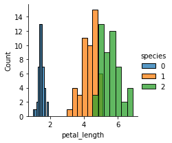
sns.FacetGrid(iris,hue="species", height=3).map(sns.histplot,"petal_length").add_legend()
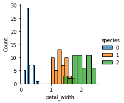
sns.FacetGrid(iris,hue="species", height=3).map(sns.histplot,"petal_width").add_legend()
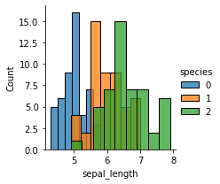
sns.FacetGrid(iris,hue="species", height=3).map(sns.histplot,"sepal_length").add_legend()
plt.show()
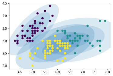
For a more concise visualization later, we just select sepal_length and sepal_width as the input variables.
X = iris.iloc[:, [0, 1]].values
y = iris.iloc[:, 4]
11.2.4.1. Training GMM
from sklearn.mixture import GaussianMixture

GMM = GaussianMixture(n_components = 3)
GMM.fit(X)
GaussianMixture(n_components=3)
11.2.4.2. Results
We can plot the Gaussians by using a plot_gmm function defined on
https://jakevdp.github.io/PythonDataScienceHandbook/05.12-gaussian-mixtures.html.
from matplotlib.patches import Ellipse

def draw_ellipse(position, covariance, ax=None, **kwargs):
    """Draw an ellipse with a given position and covariance"""
    ax = ax or plt.gca()

    # Convert covariance to principal axes
    if covariance.shape == (2, 2):
        U, s, Vt = np.linalg.svd(covariance)
        angle = np.degrees(np.arctan2(U[1, 0], U[0, 0]))
        width, height = 2 * np.sqrt(s)
    else:
        angle = 0
        width, height = 2 * np.sqrt(covariance)

    # Draw the Ellipse
    for nsig in range(1, 4):
        ax.add_patch(Ellipse(position, nsig * width, nsig * height,
                             angle, **kwargs))

def plot_gmm(gmm, X, label=True, ax=None):
    ax = ax or plt.gca()
    labels = gmm.predict(X)
    if label:
        ax.scatter(X[:, 0], X[:, 1], c=labels, s=40, cmap='viridis', zorder=2)
    else:
        ax.scatter(X[:, 0], X[:, 1], s=40, zorder=2)
    ax.axis('equal')

    w_factor = 0.2 / gmm.weights_.max()
    for pos, covar, w in zip(gmm.means_, gmm.covariances_, gmm.weights_):
        draw_ellipse(pos, covar, alpha=w * w_factor)
plot_gmm(GMM, X)
# print the converged log-likelihood value
print(GMM.lower_bound_)

# print the number of iterations needed
# for the log-likelihood value to converge
print(GMM.n_iter_)
-1.4987505566235162
8
11.2.4.3. Prediction
If we have some new data, we can use GMM.predict to predict which Gaussian they belong to.
from numpy.random import choice
from numpy.random import multivariate_normal

# first choose the clusters for 4 new data points
draw = choice(range(3), 4, p=GMM.weights_)

# sample the new data points within their chosen cluster
sample_test=[]
for i in range(len(draw)):
    n = draw[i]
    sample_test.append(
        multivariate_normal(GMM.means_[n],GMM.covariances_[n]))
GMM.predict(sample_test)
array([1, 1, 0, 1])
11.2.5. Comparison to K-means
Both GMM and K-means are unsupervised clustering models, but GMM seems to be more robust as it introduces probabilities. However, GMM is generally slower than K-Means because it takes more iterations to converge. GMM can also quickly converge to a local minimum, not the optimal solution.
In practice, GMM can be initialized by K-Means centroids to speed up the convergence.