Ridge Regression
Contents
9.7. Ridge Regression
Ridge regression is a method of linear regression that helps prevent overfitting a model in the case of high correlation between variables. It is a regularization method - a method specifically designed to reduce overfitting a model.
While OLS regression minimizes the Residual Sum of Squares, Ridge regression is the Residual Sum Squares + Shrinkage Penalty: \(λΣβj^2\)
A larger λ means a harsher penalty and smaller coefficients, but at a certain point, the coefficients will become underestimated, greatly increasing bias in the model. Following the variance-bias tradeoff, the λ chosen must be one that introduces some bias while minimizing the variance and MSE.
Basic Steps (for models with known multicollinearity):
Standardize each predictor variable
Fit model and choose λ (either through ridge trace plot or MSE of each λ)
Test model accuracy
Biggest Drawback: no variable selection = final model includes all predictors
makes coefficients very close to 0 if not significant
Better predictions, but harder to interpret
good for models where most/all variables significant
9.7.1. In Python
The Ridge and RidgeCV () are availble through sklearn.linear_model
RidgeCV:
Ridge with a cross-validation option
import pandas as pd
import seaborn as sns

flowers = sns.load_dataset('iris')
flowers = flowers.drop(['species'], axis = 1)
flowers.head()
| sepal_length | sepal_width | petal_length | petal_width | |
|---|---|---|---|---|
| 0 | 5.1 | 3.5 | 1.4 | 0.2 |
| 1 | 4.9 | 3.0 | 1.4 | 0.2 |
| 2 | 4.7 | 3.2 | 1.3 | 0.2 |
| 3 | 4.6 | 3.1 | 1.5 | 0.2 |
| 4 | 5.0 | 3.6 | 1.4 | 0.2 |
import matplotlib.pyplot as plt

flowers_corr = flowers.corr()
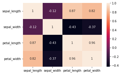
sns.heatmap(flowers_corr, annot = True)
plt.show

flowers_corr
| sepal_length | sepal_width | petal_length | petal_width | |
|---|---|---|---|---|
| sepal_length | 1.000000 | -0.117570 | 0.871754 | 0.817941 |
| sepal_width | -0.117570 | 1.000000 | -0.428440 | -0.366126 |
| petal_length | 0.871754 | -0.428440 | 1.000000 | 0.962865 |
| petal_width | 0.817941 | -0.366126 | 0.962865 | 1.000000 |

from sklearn.linear_model import Ridge
from sklearn.preprocessing import StandardScaler
from sklearn.model_selection import train_test_split
X = flowers[['sepal_length', 'petal_width', 'petal_length']]
y = flowers['sepal_width']

scaler = StandardScaler()
Xs = scaler.fit_transform(X)

X_train, X_test, y_train, y_test = train_test_split(X, y, test_size = 0.25, random_state = 0)

model = Ridge()

model.fit(X_train, y_train)

y_pred = model.predict(X_test)
from sklearn.metrics import r2_score

print(r2_score(y_test, y_pred))
0.5310770203976505
Then we run the model again using regular OLS regression.
from statsmodels.formula.api import ols
model2 = ols('sepal_width ~ sepal_length + petal_width + petal_length', data = flowers)

fit2 = model2.fit()
fit2.summary()
| Dep. Variable: | sepal_width | R-squared: | 0.524 |
|---|---|---|---|
| Model: | OLS | Adj. R-squared: | 0.514 |
| Method: | Least Squares | F-statistic: | 53.58 |
| Date: | Fri, 29 Jul 2022 | Prob (F-statistic): | 2.06e-23 |
| Time: | 22:52:36 | Log-Likelihood: | -32.100 |
| No. Observations: | 150 | AIC: | 72.20 |
| Df Residuals: | 146 | BIC: | 84.24 |
| Df Model: | 3 | ||
| Covariance Type: | nonrobust |
| coef | std err | t | P>|t| | [0.025 | 0.975] | |
|---|---|---|---|---|---|---|
| Intercept | 1.0431 | 0.271 | 3.855 | 0.000 | 0.508 | 1.578 |
| sepal_length | 0.6071 | 0.062 | 9.765 | 0.000 | 0.484 | 0.730 |
| petal_width | 0.5580 | 0.123 | 4.553 | 0.000 | 0.316 | 0.800 |
| petal_length | -0.5860 | 0.062 | -9.431 | 0.000 | -0.709 | -0.463 |
| Omnibus: | 0.738 | Durbin-Watson: | 1.889 |
|---|---|---|---|
| Prob(Omnibus): | 0.691 | Jarque-Bera (JB): | 0.426 |
| Skew: | -0.102 | Prob(JB): | 0.808 |
| Kurtosis: | 3.163 | Cond. No. | 82.1 |
Notes:
[1] Standard Errors assume that the covariance matrix of the errors is correctly specified.
The R-squared value is 0.524, so for this particular model, multicollinearity does not appear to have a significant effect.