Cartopy
Contents
8.3. Cartopy
Cartopy is a python library that can be used in combination with matplotlib to create geographical maps.
Starting in 2016, The Cartopy Project began development as a replacement for Basemap.
Cartopy has 28 people listed as contributors.
If you use conda, cartopy can be installed with
conda install -c conda-forge cartopy, which takes care of the
dependencies such as proj, geos, pyshp, shapely, etc.
If you use pip, the system dependencies need to be installed first
before running pip install cartopy. See
https://scitools.org.uk/cartopy/docs/latest/installing.html
for detailed instructions.
Pros of Cartopy:
Relatively easy to learn
Many different types of mapping projections
Great options to color in the map
Cons of Cartopy:
Slow loading times for complex maps
Alternate files often required for high precision mapping
Sources:
https://matplotlib.org/basemap/
https://scitools.org.uk/cartopy/docs/latest/
https://www.youtube.com/watch?v=4M2aiHvhr5Y
import cartopy
import cartopy.crs as ccrs
import cartopy.feature as cfeature
import cartopy.io.shapereader as shpreader
import matplotlib.pyplot as plt
import pandas as pd
import numpy as np
import seaborn as sns
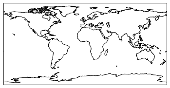
8.3.1. Basic Plot
To create a cartopy plot, simply set a variable (m for map) to plt.axes() with a projection argument.
Then add coastlines so the graph has a visible element.
m = plt.axes(projection=ccrs.PlateCarree())
m.coastlines()
<cartopy.mpl.feature_artist.FeatureArtist at 0x7f6f624c7d00>
/home/runner/work/ids-s22/ids-s22/env/lib/python3.9/site-packages/cartopy/io/__init__.py:241: DownloadWarning: Downloading: https://naciscdn.org/naturalearth/110m/physical/ne_110m_coastline.zip
  warnings.warn('Downloading: {}'.format(url), DownloadWarning)
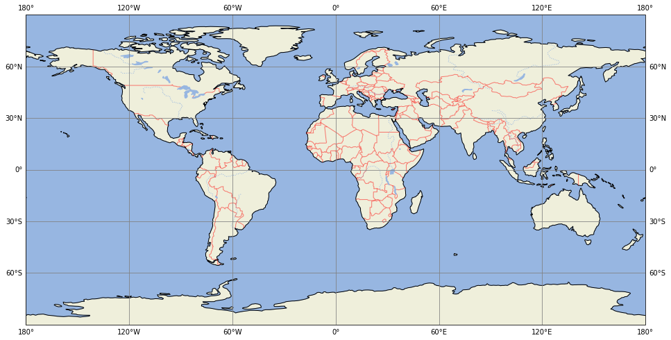
8.3.2. Advanced Graph
By using add_feature, we can add more geographic information to our graph.
gridlines will add longitude and latitude lines to the graph.
plt.figure(figsize=(16,12))
m = plt.axes(projection=ccrs.PlateCarree())

m.add_feature(cfeature.LAND)
m.add_feature(cfeature.OCEAN)
m.add_feature(cfeature.COASTLINE)
m.add_feature(cfeature.BORDERS, color = "red", alpha = 0.5)
m.add_feature(cfeature.LAKES)
m.add_feature(cfeature.RIVERS, linestyle = ':')

m.gridlines(draw_labels=True, color = "gray")
<cartopy.mpl.gridliner.Gridliner at 0x7f6f1e841eb0>
/home/runner/work/ids-s22/ids-s22/env/lib/python3.9/site-packages/cartopy/mpl/gridliner.py:549: ShapelyDeprecationWarning: __len__ for multi-part geometries is deprecated and will be removed in Shapely 2.0. Check the length of the `geoms` property instead to get the  number of parts of a multi-part geometry.
  elif len(intersection) > 4:
/home/runner/work/ids-s22/ids-s22/env/lib/python3.9/site-packages/cartopy/mpl/gridliner.py:556: ShapelyDeprecationWarning: __getitem__ for multi-part geometries is deprecated and will be removed in Shapely 2.0. Use the `geoms` property to access the constituent parts of a multi-part geometry.
  xy = np.append(intersection[0], intersection[-1],
<__array_function__ internals>:5: ShapelyDeprecationWarning: The array interface is deprecated and will no longer work in Shapely 2.0. Convert the '.coords' to a numpy array instead.
/home/runner/work/ids-s22/ids-s22/env/lib/python3.9/site-packages/numpy/lib/function_base.py:4817: ShapelyDeprecationWarning: The array interface is deprecated and will no longer work in Shapely 2.0. Convert the '.coords' to a numpy array instead.
  return concatenate((arr, values), axis=axis)
/home/runner/work/ids-s22/ids-s22/env/lib/python3.9/site-packages/cartopy/io/__init__.py:241: DownloadWarning: Downloading: https://naciscdn.org/naturalearth/110m/physical/ne_110m_land.zip
  warnings.warn('Downloading: {}'.format(url), DownloadWarning)
/home/runner/work/ids-s22/ids-s22/env/lib/python3.9/site-packages/cartopy/io/__init__.py:241: DownloadWarning: Downloading: https://naciscdn.org/naturalearth/110m/physical/ne_110m_ocean.zip
  warnings.warn('Downloading: {}'.format(url), DownloadWarning)
/home/runner/work/ids-s22/ids-s22/env/lib/python3.9/site-packages/cartopy/io/__init__.py:241: DownloadWarning: Downloading: https://naciscdn.org/naturalearth/110m/cultural/ne_110m_admin_0_boundary_lines_land.zip
  warnings.warn('Downloading: {}'.format(url), DownloadWarning)
/home/runner/work/ids-s22/ids-s22/env/lib/python3.9/site-packages/cartopy/mpl/style.py:76: UserWarning: facecolor will have no effect as it has been defined as "never".
  warnings.warn('facecolor will have no effect as it has been '
/home/runner/work/ids-s22/ids-s22/env/lib/python3.9/site-packages/cartopy/io/__init__.py:241: DownloadWarning: Downloading: https://naciscdn.org/naturalearth/110m/physical/ne_110m_lakes.zip
  warnings.warn('Downloading: {}'.format(url), DownloadWarning)
/home/runner/work/ids-s22/ids-s22/env/lib/python3.9/site-packages/cartopy/io/__init__.py:241: DownloadWarning: Downloading: https://naciscdn.org/naturalearth/110m/physical/ne_110m_rivers_lake_centerlines.zip
  warnings.warn('Downloading: {}'.format(url), DownloadWarning)
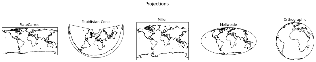
8.3.3. Projection Comparison
Here are some examples of different projections.
fig = plt.figure(figsize=(20,20))
fig.suptitle('Projections', fontsize = 15, y = 0.93)

projections = {'PlateCarree': ccrs.PlateCarree(),
               'EquidistantConic': ccrs.EquidistantConic(),
               'Miller': ccrs.Miller(),
               'Mollweide': ccrs.Mollweide(),
               'Orthographic': ccrs.Orthographic()}

for index, projection in enumerate(projections.items()):
    ax = fig.add_subplot(7, 5, index+1, projection=projection[1])
    ax.coastlines()
    ax.set_title(projection[0])
/home/runner/work/ids-s22/ids-s22/env/lib/python3.9/site-packages/cartopy/crs.py:228: ShapelyDeprecationWarning: __len__ for multi-part geometries is deprecated and will be removed in Shapely 2.0. Check the length of the `geoms` property instead to get the  number of parts of a multi-part geometry.
  if len(multi_line_string) > 1:
/home/runner/work/ids-s22/ids-s22/env/lib/python3.9/site-packages/cartopy/crs.py:280: ShapelyDeprecationWarning: Iteration over multi-part geometries is deprecated and will be removed in Shapely 2.0. Use the `geoms` property to access the constituent parts of a multi-part geometry.
  for line in multi_line_string:
/home/runner/work/ids-s22/ids-s22/env/lib/python3.9/site-packages/cartopy/crs.py:347: ShapelyDeprecationWarning: __len__ for multi-part geometries is deprecated and will be removed in Shapely 2.0. Check the length of the `geoms` property instead to get the  number of parts of a multi-part geometry.
  if len(p_mline) > 0:
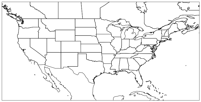
8.3.4. Plotting Specific Locations
If you only want to plot a certain area of the map, you can specify set_extent.
To do this, specify a list of points [lowest longitude, highest longitude, lowest latidude, highest latitude]
as well as the projection (optionally).
fig = plt.figure(figsize=(14, 14))
m = plt.axes(projection=ccrs.PlateCarree())
# (x0, x1, y0, y1)
m.set_extent([-130, -60, 20, 55], ccrs.PlateCarree())
m.add_feature(cfeature.STATES)
m.coastlines()
<cartopy.mpl.feature_artist.FeatureArtist at 0x7f6f1e698ac0>
/home/runner/work/ids-s22/ids-s22/env/lib/python3.9/site-packages/cartopy/io/__init__.py:241: DownloadWarning: Downloading: https://naciscdn.org/naturalearth/50m/cultural/ne_50m_admin_1_states_provinces_lakes.zip
  warnings.warn('Downloading: {}'.format(url), DownloadWarning)
/home/runner/work/ids-s22/ids-s22/env/lib/python3.9/site-packages/cartopy/io/__init__.py:241: DownloadWarning: Downloading: https://naciscdn.org/naturalearth/50m/physical/ne_50m_coastline.zip
  warnings.warn('Downloading: {}'.format(url), DownloadWarning)
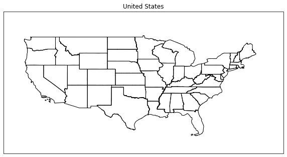
8.3.5. Reading Shape Files
If you would like to plot one area without the adjacent landscape,
you can use a shape file via Reader from cartopy.io.shapereader.
# get shape file
reader = shpreader.Reader('../data/state/tl_2021_us_state.dbf')

# convert shape file to format that cartopy can work with
states = list(reader.geometries())
STATES = cfeature.ShapelyFeature(states, ccrs.PlateCarree())

# create plot
plt.figure(figsize=(10, 6))
m = plt.axes(projection=ccrs.PlateCarree())
plt.title("United States")
m.set_extent([-130, -60, 20, 50])
m.add_feature(STATES, facecolor='none', edgecolor='black')
<cartopy.mpl.feature_artist.FeatureArtist at 0x7f6f1cf1ea00>
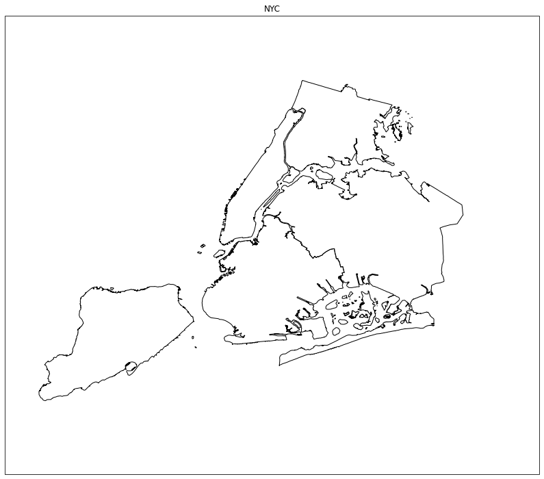
Here is a plot of New York City that we will use later.
# get shape file
reader = shpreader.Reader('../data/nyc/geo_export_a1f96cd2-7ce6-44bb-9568-f3ee8bcba44a.dbf')

# convert shape file to format that cartopy can work with
geom = list(reader.geometries())
GEOM = cfeature.ShapelyFeature(geom, ccrs.PlateCarree())

# create plot
plt.figure(figsize=(14, 14))
m = plt.axes(projection=ccrs.PlateCarree())
plt.title("NYC")
m.set_extent([-74.3, -73.6, 40.4, 41])
m.add_feature(GEOM, facecolor='none', edgecolor='black')
<cartopy.mpl.feature_artist.FeatureArtist at 0x7f6f1e5644f0>
8.3.6. Data Cleaning
Before we can work with the NYC Collisions Dataset, we need to do some data cleaning.
df = pd.read_csv("../data/nyc_mv_collisions_202201.csv")
print(df.shape)
df.head()
(7659, 29)
| CRASH DATE | CRASH TIME | BOROUGH | ZIP CODE | LATITUDE | LONGITUDE | LOCATION | ON STREET NAME | CROSS STREET NAME | OFF STREET NAME | ... | CONTRIBUTING FACTOR VEHICLE 2 | CONTRIBUTING FACTOR VEHICLE 3 | CONTRIBUTING FACTOR VEHICLE 4 | CONTRIBUTING FACTOR VEHICLE 5 | COLLISION_ID | VEHICLE TYPE CODE 1 | VEHICLE TYPE CODE 2 | VEHICLE TYPE CODE 3 | VEHICLE TYPE CODE 4 | VEHICLE TYPE CODE 5 | |
|---|---|---|---|---|---|---|---|---|---|---|---|---|---|---|---|---|---|---|---|---|---|
| 0 | 01/01/2022 | 7:05 | NaN | NaN | NaN | NaN | NaN | EAST 128 STREET | 3 AVENUE BRIDGE | NaN | ... | NaN | NaN | NaN | NaN | 4491172 | Sedan | NaN | NaN | NaN | NaN |
| 1 | 01/01/2022 | 14:43 | NaN | NaN | 40.769993 | -73.915825 | (40.769993, -73.915825) | GRAND CENTRAL PKWY | NaN | NaN | ... | NaN | NaN | NaN | NaN | 4491406 | Sedan | Sedan | NaN | NaN | NaN |
| 2 | 01/01/2022 | 21:20 | QUEENS | 11414.0 | 40.657230 | -73.841380 | (40.65723, -73.84138) | 91 STREET | 160 AVENUE | NaN | ... | NaN | NaN | NaN | NaN | 4491466 | Sedan | NaN | NaN | NaN | NaN |
| 3 | 01/01/2022 | 4:30 | NaN | NaN | NaN | NaN | NaN | Southern parkway | Jfk expressway | NaN | ... | Unspecified | NaN | NaN | NaN | 4491626 | Sedan | Sedan | NaN | NaN | NaN |
| 4 | 01/01/2022 | 7:57 | NaN | NaN | NaN | NaN | NaN | WESTCHESTER AVENUE | SHERIDAN EXPRESSWAY | NaN | ... | NaN | NaN | NaN | NaN | 4491734 | Sedan | NaN | NaN | NaN | NaN |
5 rows × 29 columns
As we can see from the plot below, there are some issues with our dataset.
sns.scatterplot(x="LONGITUDE", y="LATITUDE", data=df, hue = "BOROUGH")
<AxesSubplot:xlabel='LONGITUDE', ylabel='LATITUDE'>
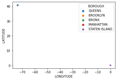
Some points have the coordinates (0, 0) so we need to remove them from the dataset.
We can also remove the rows in which the longitude/latitude data is missing.
# drop rows with longitude == 0
df[df.LONGITUDE == 0] = np.nan

# make sure bad latitude values are all removed now
print(df.LATITUDE.isna().sum())
print(df.loc[df.LATITUDE == 0].shape[0])

df.head()
582
0
| CRASH DATE | CRASH TIME | BOROUGH | ZIP CODE | LATITUDE | LONGITUDE | LOCATION | ON STREET NAME | CROSS STREET NAME | OFF STREET NAME | ... | CONTRIBUTING FACTOR VEHICLE 2 | CONTRIBUTING FACTOR VEHICLE 3 | CONTRIBUTING FACTOR VEHICLE 4 | CONTRIBUTING FACTOR VEHICLE 5 | COLLISION_ID | VEHICLE TYPE CODE 1 | VEHICLE TYPE CODE 2 | VEHICLE TYPE CODE 3 | VEHICLE TYPE CODE 4 | VEHICLE TYPE CODE 5 | |
|---|---|---|---|---|---|---|---|---|---|---|---|---|---|---|---|---|---|---|---|---|---|
| 0 | 01/01/2022 | 7:05 | NaN | NaN | NaN | NaN | NaN | EAST 128 STREET | 3 AVENUE BRIDGE | NaN | ... | NaN | NaN | NaN | NaN | 4491172.0 | Sedan | NaN | NaN | NaN | NaN |
| 1 | 01/01/2022 | 14:43 | NaN | NaN | 40.769993 | -73.915825 | (40.769993, -73.915825) | GRAND CENTRAL PKWY | NaN | NaN | ... | NaN | NaN | NaN | NaN | 4491406.0 | Sedan | Sedan | NaN | NaN | NaN |
| 2 | 01/01/2022 | 21:20 | QUEENS | 11414.0 | 40.657230 | -73.841380 | (40.65723, -73.84138) | 91 STREET | 160 AVENUE | NaN | ... | NaN | NaN | NaN | NaN | 4491466.0 | Sedan | NaN | NaN | NaN | NaN |
| 3 | 01/01/2022 | 4:30 | NaN | NaN | NaN | NaN | NaN | Southern parkway | Jfk expressway | NaN | ... | Unspecified | NaN | NaN | NaN | 4491626.0 | Sedan | Sedan | NaN | NaN | NaN |
| 4 | 01/01/2022 | 7:57 | NaN | NaN | NaN | NaN | NaN | WESTCHESTER AVENUE | SHERIDAN EXPRESSWAY | NaN | ... | NaN | NaN | NaN | NaN | 4491734.0 | Sedan | NaN | NaN | NaN | NaN |
5 rows × 29 columns
df.info()
<class 'pandas.core.frame.DataFrame'>
RangeIndex: 7659 entries, 0 to 7658
Data columns (total 29 columns):
 #   Column                         Non-Null Count  Dtype
---  ------                         --------------  -----
 0   CRASH DATE                     7639 non-null   object
 1   CRASH TIME                     7639 non-null   object
 2   BOROUGH                        5010 non-null   object
 3   ZIP CODE                       5010 non-null   float64
 4   LATITUDE                       7077 non-null   float64
 5   LONGITUDE                      7077 non-null   float64
 6   LOCATION                       7077 non-null   object
 7   ON STREET NAME                 5607 non-null   object
 8   CROSS STREET NAME              3606 non-null   object
 9   OFF STREET NAME                2032 non-null   object
 10  NUMBER OF PERSONS INJURED      7639 non-null   float64
 11  NUMBER OF PERSONS KILLED       7639 non-null   float64
 12  NUMBER OF PEDESTRIANS INJURED  7639 non-null   float64
 13  NUMBER OF PEDESTRIANS KILLED   7639 non-null   float64
 14  NUMBER OF CYCLIST INJURED      7639 non-null   float64
 15  NUMBER OF CYCLIST KILLED       7639 non-null   float64
 16  NUMBER OF MOTORIST INJURED     7639 non-null   float64
 17  NUMBER OF MOTORIST KILLED      7639 non-null   float64
 18  CONTRIBUTING FACTOR VEHICLE 1  7595 non-null   object
 19  CONTRIBUTING FACTOR VEHICLE 2  5611 non-null   object
 20  CONTRIBUTING FACTOR VEHICLE 3  822 non-null    object
 21  CONTRIBUTING FACTOR VEHICLE 4  224 non-null    object
 22  CONTRIBUTING FACTOR VEHICLE 5  79 non-null     object
 23  COLLISION_ID                   7639 non-null   float64
 24  VEHICLE TYPE CODE 1            7519 non-null   object
 25  VEHICLE TYPE CODE 2            4738 non-null   object
 26  VEHICLE TYPE CODE 3            750 non-null    object
 27  VEHICLE TYPE CODE 4            206 non-null    object
 28  VEHICLE TYPE CODE 5            77 non-null     object
dtypes: float64(12), object(17)
memory usage: 1.7+ MB
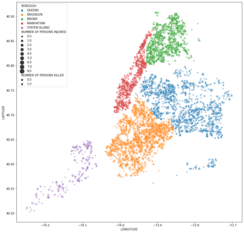
We can create a plot to show that our data has been successfully cleaned.
# specify the size of the plot
fig = plt.figure(figsize=(14, 14))

# use seaborn to plot the points
# x and y are just the longitude and latitude from the plot
# data is the dataframe, which tells seaborn to refernce the dataframe for the rest of the arguments
# hue categorizes the colors and style changes the marker to an x if someone was killed
# alpha = 0.5 makes the markers 50% transparent
# size changes the size of the point based on the amount of injuries
# for sizes, I used list concatenation to make each point 25 times bigger
sns.scatterplot(x="LONGITUDE", y="LATITUDE", data=df,
                hue = 'BOROUGH', style = "NUMBER OF PERSONS KILLED", alpha = 0.5,
                size = "NUMBER OF PERSONS INJURED",
                sizes = [(i+1)*25 for i in range(int(max(df["NUMBER OF PERSONS INJURED"] + 1)))])
<AxesSubplot:xlabel='LONGITUDE', ylabel='LATITUDE'>
8.3.7. Plotting On Cartopy Map
Using our dataset, we can plot the car crashes on their geographical location.
# specify the size of the plot
fig = plt.figure(figsize=(14, 14))

# plot on top of geographical coordinates
m = plt.axes(projection=ccrs.PlateCarree())

# set title
plt.title("Crashes in New York City (January 2022)")

# set geographical location of graph
m.set_extent([np.nanmin(df.LONGITUDE) - 0.01, np.nanmax(df.LONGITUDE) + 0.01,
              np.nanmin(df.LATITUDE) - 0.01, np.nanmax(df.LATITUDE) + 0.01], ccrs.PlateCarree())

# color in the land (the color is just a hex code for a yellow that I though looked good as land)
m.add_feature(cfeature.LAND, color = "#F3E5AB")

# color in the ocean (colors as blue by default)
m.add_feature(cfeature.OCEAN)

# use seaborn to plot the points
sns.scatterplot(x="LONGITUDE", y="LATITUDE", data=df,
                hue = 'BOROUGH', style = "NUMBER OF PERSONS KILLED", alpha = 0.5,
                size = "NUMBER OF PERSONS INJURED",
                sizes = [(i+1)*25 for i in range(int(max(df["NUMBER OF PERSONS INJURED"] + 1)))])

# if needed, you can add plt.legend(loc = "...") to change the location of the legend

# draw coastlines
m.coastlines()
<cartopy.mpl.feature_artist.FeatureArtist at 0x7f6f1e5be640>
/home/runner/work/ids-s22/ids-s22/env/lib/python3.9/site-packages/cartopy/io/__init__.py:241: DownloadWarning: Downloading: https://naciscdn.org/naturalearth/10m/physical/ne_10m_land.zip
  warnings.warn('Downloading: {}'.format(url), DownloadWarning)
/home/runner/work/ids-s22/ids-s22/env/lib/python3.9/site-packages/cartopy/io/__init__.py:241: DownloadWarning: Downloading: https://naciscdn.org/naturalearth/10m/physical/ne_10m_ocean.zip
  warnings.warn('Downloading: {}'.format(url), DownloadWarning)
/home/runner/work/ids-s22/ids-s22/env/lib/python3.9/site-packages/cartopy/io/__init__.py:241: DownloadWarning: Downloading: https://naciscdn.org/naturalearth/10m/physical/ne_10m_coastline.zip
  warnings.warn('Downloading: {}'.format(url), DownloadWarning)
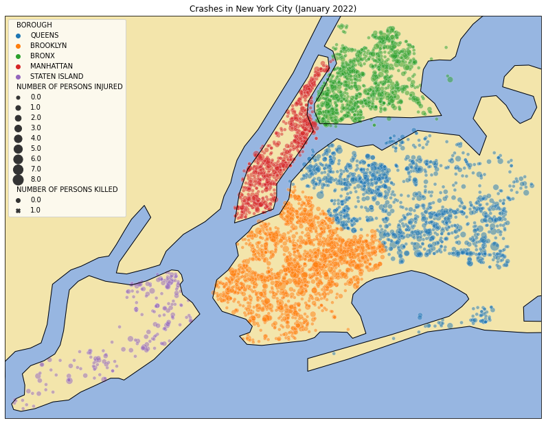
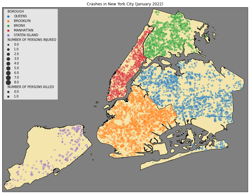
8.3.8. Plotting On Cartopy Map Using Shapefile
By making use of a shapefile, we can map with greater precision and omit the locations that are not included in our graph.
# get shape file
reader = shpreader.Reader('../data/nyc/geo_export_a1f96cd2-7ce6-44bb-9568-f3ee8bcba44a.dbf')

# convert shape file to format that cartopy can work with
geom = list(reader.geometries())
GEOM = cfeature.ShapelyFeature(geom, ccrs.PlateCarree())

# specify the size of the plot
plt.figure(figsize=(14, 14))

# plot on top of geographical coordinates
m = plt.axes(projection=ccrs.PlateCarree())

# make the default color of the plot gray (this ends up just being the background)
m.set_facecolor("gray")

# set title
plt.title("Crashes in New York City (January 2022)")

# set geographical location of graph
m.set_extent([np.nanmin(df.LONGITUDE) - 0.01, np.nanmax(df.LONGITUDE) + 0.01,
              np.nanmin(df.LATITUDE) - 0.01, np.nanmax(df.LATITUDE) + 0.01], ccrs.PlateCarree())

# add the in the New York City geography that was originally read in as a shape file
m.add_feature(GEOM, facecolor = "#F3E5AB", edgecolor='black')

# use seaborn to plot the points
# setting zorder to a high number makes it so the geography does not cover up the points
sns.scatterplot(x="LONGITUDE", y="LATITUDE", data=df,
                hue = 'BOROUGH', style = "NUMBER OF PERSONS KILLED", alpha = 0.5,
                size = "NUMBER OF PERSONS INJURED",
                sizes = [(i+1)*25 for i in range(int(max(df["NUMBER OF PERSONS INJURED"] + 1)))],
                zorder = 100)

# if needed, you can add plt.legend(loc = "...") to change the location of the legend
<GeoAxesSubplot:title={'center':'Crashes in New York City (January 2022)'}, xlabel='LONGITUDE', ylabel='LATITUDE'>