Linear and Generalized Linear Models
Contents
9.3. Linear and Generalized Linear Models
Let’s simulate some data for illustrations.
import numpy as np
import statsmodels.api as sm

nobs = 200
ncov = 5
np.random.seed(123)
x = np.random.random((nobs, ncov)) # Uniform over [0, 1)
beta = np.repeat(1, ncov)
y = 2 + np.dot(x, beta) + np.random.normal(size = nobs)
y.shape
(200,)
x.shape
(200, 5)
That is, the true linear regression model is
A regression model for the observed data can be fitted as
xmat = sm.add_constant(x)
mymod = sm.OLS(y, xmat)
myfit = mymod.fit()
myfit.summary()
| Dep. Variable: | y | R-squared: | 0.309 |
|---|---|---|---|
| Model: | OLS | Adj. R-squared: | 0.292 |
| Method: | Least Squares | F-statistic: | 17.38 |
| Date: | Fri, 29 Jul 2022 | Prob (F-statistic): | 3.31e-14 |
| Time: | 22:52:58 | Log-Likelihood: | -272.91 |
| No. Observations: | 200 | AIC: | 557.8 |
| Df Residuals: | 194 | BIC: | 577.6 |
| Df Model: | 5 | ||
| Covariance Type: | nonrobust |
| coef | std err | t | P>|t| | [0.025 | 0.975] | |
|---|---|---|---|---|---|---|
| const | 1.8754 | 0.282 | 6.656 | 0.000 | 1.320 | 2.431 |
| x1 | 1.1703 | 0.248 | 4.723 | 0.000 | 0.682 | 1.659 |
| x2 | 0.8988 | 0.235 | 3.825 | 0.000 | 0.435 | 1.362 |
| x3 | 0.9784 | 0.238 | 4.114 | 0.000 | 0.509 | 1.448 |
| x4 | 1.3418 | 0.250 | 5.367 | 0.000 | 0.849 | 1.835 |
| x5 | 0.6027 | 0.239 | 2.519 | 0.013 | 0.131 | 1.075 |
| Omnibus: | 0.810 | Durbin-Watson: | 1.978 |
|---|---|---|---|
| Prob(Omnibus): | 0.667 | Jarque-Bera (JB): | 0.903 |
| Skew: | -0.144 | Prob(JB): | 0.637 |
| Kurtosis: | 2.839 | Cond. No. | 8.31 |
Notes:
[1] Standard Errors assume that the covariance matrix of the errors is correctly specified.
How are the regression coefficients interpreted? Intercept?
Why does it make sense to center the covariates?
Now we form a data frame with the variables
import pandas as pd
df = np.concatenate((y.reshape((nobs, 1)), x), axis = 1)
df = pd.DataFrame(data = df,
                  columns = ["y"] + ["x" + str(i) for i in range(1,
                  ncov + 1)])
df.info()
<class 'pandas.core.frame.DataFrame'>
RangeIndex: 200 entries, 0 to 199
Data columns (total 6 columns):
 #   Column  Non-Null Count  Dtype
---  ------  --------------  -----
 0   y       200 non-null    float64
 1   x1      200 non-null    float64
 2   x2      200 non-null    float64
 3   x3      200 non-null    float64
 4   x4      200 non-null    float64
 5   x5      200 non-null    float64
dtypes: float64(6)
memory usage: 9.5 KB
Let’s use a formula to specify the regression model as in R, and fit
a robust linear model (rlm) instead of OLS.
import statsmodels.formula.api as smf
mymod = smf.rlm(formula = "y ~ x1 + x2 + x3 + x4 + x5", data = df)
myfit = mymod.fit()
myfit.summary()
| Dep. Variable: | y | No. Observations: | 200 |
|---|---|---|---|
| Model: | RLM | Df Residuals: | 194 |
| Method: | IRLS | Df Model: | 5 |
| Norm: | HuberT | ||
| Scale Est.: | mad | ||
| Cov Type: | H1 | ||
| Date: | Fri, 29 Jul 2022 | ||
| Time: | 22:52:58 | ||
| No. Iterations: | 16 |
| coef | std err | z | P>|z| | [0.025 | 0.975] | |
|---|---|---|---|---|---|---|
| Intercept | 1.8353 | 0.294 | 6.246 | 0.000 | 1.259 | 2.411 |
| x1 | 1.1254 | 0.258 | 4.355 | 0.000 | 0.619 | 1.632 |
| x2 | 0.9664 | 0.245 | 3.944 | 0.000 | 0.486 | 1.447 |
| x3 | 0.9995 | 0.248 | 4.029 | 0.000 | 0.513 | 1.486 |
| x4 | 1.3275 | 0.261 | 5.091 | 0.000 | 0.816 | 1.839 |
| x5 | 0.6768 | 0.250 | 2.712 | 0.007 | 0.188 | 1.166 |
If the model instance has been used for another fit with different fit parameters, then the fit options might not be the correct ones anymore .
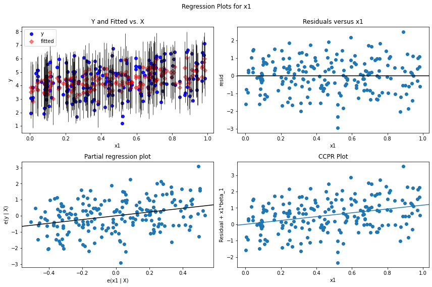
For model diagnostics, one can check residual plots.
import matplotlib.pyplot as plt

myOlsFit = smf.ols(formula = "y ~ x1 + x2 + x3 + x4 + x5", data = df).fit()
fig = plt.figure(figsize = (12, 8))
## residual versus x1; can do the same for other covariates
fig = sm.graphics.plot_regress_exog(myOlsFit, 'x1', fig=fig)
eval_env: 1
See more on residual diagnostics and specification tests.
9.4. Generalized Linear Regression
A linear regression model cannot be applied to presence/absence or count data.
Binary or count data need to be modeled under a generlized framework. Consider a binary or count variable \(Y\) with possible covariates \(X\). A generalized model describes a transformation \(g\) of the conditional mean \(E[Y | X]\) by a linear predictor \(X^{\top}\beta\). That is
The transformation \(g\) is known as the link function.
For logistic regression with binary outcomes, the link function is the logit function
What is the interpretation of the regression coefficients in a logistic regression? Intercept?
A logistic regression can be fit with statsmodels.api.glm.
Let’s generate some binary data first by dichotomizing existing variables.
df['yb' ] = np.where(df['y' ] > 2.5, 1, 0)
df['x1b'] = np.where(df['x1'] > 0.5, 1, 0)
Fit a logistic regression for y1b.
mylogistic = smf.glm(formula = 'yb ~ x1b + x2 + x3 + x4 + x5', data = df,
                     family = sm.families.Binomial())
mylfit = mylogistic.fit()
mylfit.summary()
| Dep. Variable: | yb | No. Observations: | 200 |
|---|---|---|---|
| Model: | GLM | Df Residuals: | 194 |
| Model Family: | Binomial | Df Model: | 5 |
| Link Function: | Logit | Scale: | 1.0000 |
| Method: | IRLS | Log-Likelihood: | -30.654 |
| Date: | Fri, 29 Jul 2022 | Deviance: | 61.307 |
| Time: | 22:53:00 | Pearson chi2: | 217. |
| No. Iterations: | 7 | Pseudo R-squ. (CS): | 0.05871 |
| Covariance Type: | nonrobust |
| coef | std err | z | P>|z| | [0.025 | 0.975] | |
|---|---|---|---|---|---|---|
| Intercept | -0.4354 | 1.309 | -0.333 | 0.739 | -3.002 | 2.131 |
| x1b | 1.2721 | 0.845 | 1.505 | 0.132 | -0.384 | 2.928 |
| x2 | 2.6897 | 1.418 | 1.897 | 0.058 | -0.089 | 5.469 |
| x3 | -0.0537 | 1.270 | -0.042 | 0.966 | -2.542 | 2.435 |
| x4 | 2.6576 | 1.438 | 1.848 | 0.065 | -0.160 | 5.476 |
| x5 | 1.8752 | 1.330 | 1.409 | 0.159 | -0.732 | 4.483 |
If we treat y1b as count data, a Poisson regression can be fitted.
myPois = smf.glm(formula = 'yb ~ x1b + x2 + x3 + x4 + x5', data = df,
                 family = sm.families.Poisson())
mypfit = myPois.fit()
mypfit.summary()
| Dep. Variable: | yb | No. Observations: | 200 |
|---|---|---|---|
| Model: | GLM | Df Residuals: | 194 |
| Model Family: | Poisson | Df Model: | 5 |
| Link Function: | Log | Scale: | 1.0000 |
| Method: | IRLS | Log-Likelihood: | -199.55 |
| Date: | Fri, 29 Jul 2022 | Deviance: | 17.091 |
| Time: | 22:53:00 | Pearson chi2: | 8.99 |
| No. Iterations: | 4 | Pseudo R-squ. (CS): | 0.002487 |
| Covariance Type: | nonrobust |
| coef | std err | z | P>|z| | [0.025 | 0.975] | |
|---|---|---|---|---|---|---|
| Intercept | -0.2045 | 0.288 | -0.710 | 0.477 | -0.769 | 0.360 |
| x1b | 0.0445 | 0.146 | 0.304 | 0.761 | -0.242 | 0.331 |
| x2 | 0.0965 | 0.249 | 0.387 | 0.699 | -0.392 | 0.585 |
| x3 | -0.0088 | 0.254 | -0.035 | 0.972 | -0.507 | 0.490 |
| x4 | 0.1072 | 0.267 | 0.402 | 0.688 | -0.416 | 0.630 |
| x5 | 0.0750 | 0.253 | 0.296 | 0.767 | -0.421 | 0.571 |